Lab 6: estimation (solutions)
Ben Bolker
© 2005 Ben Bolker
Exercise 1:
(Recreate negative binomial data, likelihood surface, etc.):
> set.seed(1001)
> mu.true = 1
> k.true = 0.4
> x = rnbinom(50, mu = mu.true, size = k.true)
> NLLfun1 = function(p, dat = x) {
+     mu = p[1]
+     k = p[2]
+     -sum(dnbinom(x, mu = mu, size = k, log = TRUE))
+ }
Method-of-moments estimates, for starting point:
> m = mean(x)
> v = var(x)
> mu.mom = m
> k.mom = m/(v/m - 1)
Using optim() to find best fit:
> O1 = optim(fn = NLLfun1, par = c(mu = mu.mom, k = k.mom))
> O1
$par
       mu         k
1.2602356 0.2884793

$value
[1] 71.79646

$counts
function gradient
      45       NA

$convergence
[1] 0

$message
NULL
Calculating likelihood surface:
> muvec = seq(0.4, 3, by = 0.05)
> kvec = seq(0.01, 0.7, by = 0.01)
> resmat = matrix(nrow = length(muvec), ncol = length(kvec))
> for (i in 1:length(muvec)) {
+     for (j in 1:length(kvec)) {
+         resmat[i, j] = NLLfun1(c(muvec[i], kvec[j]))
+     }
+ }
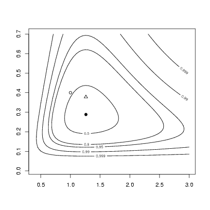
The new part: (1) construct confidence levels
(bivariate, so use df=2 in qchisq):
> alevels = c(0.5, 0.9, 0.95, 0.99, 0.999)
> minval = O1$value
> nll.levels = qchisq(alevels, df = 2)/2 + minval
Draw the contour plot, then add MLEs,
true values, and method-of-moments values
> contour(muvec, kvec, resmat, levels = nll.levels, labels = alevels)
> points(O1$par["mu"], O1$par["k"], pch = 16)
> points(mu.true, k.true, pch = 1)
> points(mu.mom, k.mom, pch = 2)
 Exercise 2:
Set up reef fish data, yet again:
> a = 0.696
> b = 9.79
> recrprob = function(x, a = 0.696, b = 9.79) a/(1 + (a/b) * x)
> scoefs = c(mu = 25.32, k = 0.932, zprob = 0.123)
> rzinbinom = function(n, mu, size, zprob) {
+     ifelse(runif(n) < zprob, 0, rnbinom(n, mu = mu, size = size))
+ }
> settlers = rzinbinom(603, mu = scoefs["mu"], size = scoefs["k"],
+     zprob = scoefs["zprob"])
> recr = rbinom(603, prob = recrprob(settlers), size = settlers)
Likelihood functions for Shepherd, BH, and constant model,
using log-scaled parameters:
> NLLfun3L = function(loga, logb, logd) {
+     a = exp(loga)
+     b = exp(logb)
+     d = exp(logd)
+     recrprob = a/(1 + (a/b) * settlers^d)
+     -sum(dbinom(recr, prob = recrprob, size = settlers, log = TRUE),
+         na.rm = TRUE)
+ }
> NLLfun4L = function(loga, logb) {
+     a = exp(loga)
+     b = exp(logb)
+     recrprob = a/(1 + (a/b) * settlers)
+     -sum(dbinom(recr, prob = recrprob, size = settlers, log = TRUE),
+         na.rm = TRUE)
+ }
> NLLfun5L = function(loga) {
+     a = exp(loga)
+     recrprob = a
+     r = -sum(dbinom(recr, prob = recrprob, size = settlers, log = TRUE),
+         na.rm = TRUE)
+     return(r)
+ }
Start by doing linear regression of recruits vs. settlers,
with a zero intercept:
> lm1 = lm(recr ~ settlers - 1)
> lm.loga = list(log(coef(lm1)))
> rename = function(L, names) {
+     for (i in seq(along = L)) {
+         names(L[[i]]) = NULL
+     }
+     names(L) = names
+     L
+ }
> lm.loga = rename(lm.loga, "loga")
First fit density-independent model, using BFGS
> library(stats4)
> m5L = mle(minuslogl = NLLfun5L, start = list(loga = -1), method = "BFGS",
+     control = list(ndeps = 0.01))
Had to use Nelder-Mead instead of BFGS:
> library(stats4)
> m4L = mle(minuslogl = NLLfun4L, start = list(loga = log(0.5),
+     logb = log(10)), method = "Nelder-Mead")
set new starting condition to coeffs of last fit:
> s3 = c(coef(m4L), list(logd = 0))
> m3L = mle(minuslogl = NLLfun3L, start = s3, method = "Nelder-Mead")
Table of coefficients and log-likelihoods:
> lin = c(exp(coef(m5L)), NA, NA, -logLik(m5L))
> BH = c(exp(coef(m4L)), NA, -logLik(m4L))
> shep = c(exp(coef(m3L)), -logLik(m3L))
> ptab = rbind(lin, BH, shep)
> colnames(ptab) = c("a", "b", "d", "NLL")
> ptab
             a        b        d      NLL
lin  0.1956194       NA       NA 1444.717
BH   0.6469000 9.661556       NA 1020.843
shep 0.6958790 7.488366 0.938981 1020.427
Confidence intervals:
> exp(confint(m3L))
Profiling...
         2.5 %     97.5 %
loga 0.5803975  0.8629401
logb 4.5138376 13.2413092
logd 0.8183324  1.0738117
> exp(confint(m4L))
Profiling...
         2.5 %     97.5 %
loga 0.5833116  0.7180536
logb 8.9412988 10.4843910
> exp(confint(m5L))
Profiling...
    2.5 %    97.5 %
0.1888597 0.2025078
Exercise 3:
ZINB, negative binomial, Poisson:
> NLLpois = function(lambda) {
+     -sum(dpois(settlers, lambda = lambda, log = TRUE))
+ }
> NLLnb = function(mu, k) {
+     -sum(dnbinom(settlers, mu = mu, size = k, log = TRUE))
+ }
Set up ZINB function again:
> dzinbinom = function(x, mu, size, zprob, log = FALSE) {
+     v = ifelse(x == 0, zprob + (1 - zprob) * dnbinom(0, mu = mu,
+         size = size), (1 - zprob) * dnbinom(x, mu = mu, size = size))
+     if (log)
+         return(log(v))
+     else v
+ }
> NLLzinb = function(mu, k, zprob) {
+     -sum(dzinbinom(settlers, mu = mu, size = k, zprob = zprob,
+         log = TRUE))
+ }
Fit all three functions, from simplest to most complex:
> m = mean(settlers)
> mpois = mle(minuslogl = NLLpois, start = list(lambda = m))
> mnbinom = mle(minuslogl = NLLnb, start = list(mu = m, k = 0.5))
> mzinbinom = mle(minuslogl = NLLzinb, start = list(mu = m, k = 0.5,
+     zprob = 0.5))
Table of coefficients and log-likelihoods:
> pois = c(coef(mpois), NA, NA, -logLik(mpois))
> nbin = c(coef(mnbinom), NA, -logLik(mnbinom))
> zinb = c(coef(mzinbinom), -logLik(mzinbinom))
> ptab = rbind(pois, nbin, zinb)
> colnames(ptab) = c("lambda/mu", "k", "zprob", "NLL")
> ptab
     lambda/mu         k     zprob      NLL
pois  21.52405        NA        NA 8623.188
nbin  21.52405 0.6238752        NA 2432.672
zinb  24.45607 1.0250050 0.1199043 2411.265
The zero-inflated negative binomial wins
by a very large margin (how small would we
have to make the data set before we couldn't
tell the difference any more?) - 6000
log-likelihood units between neg bin and
Poisson, and an additional 21 log-likelihood
units between neg bin and z-i neg bin ...
> confint(mpois)
Profiling...
   2.5 %   97.5 %
21.15587 21.89647
> confint(mnbinom)
Profiling...
        2.5 %     97.5 %
mu 19.4557009 23.8917798
k   0.5553659  0.6993166
> confint(mzinbinom)
Profiling...
            2.5 %     97.5 %
mu    22.37720768 26.7320557
k      0.87239529  1.1904082
zprob  0.08789511  0.1532577
As expected, confidence limits for m
get wider and wider as we add more parameters
to the model. Still, even zprob is
pretty well bounded from these data.
File translated from
TEX
by
TTH,
version 3.67.
On 24 Oct 2005, 18:20.
 Exercise 2:
Set up reef fish data, yet again: