The numbered problems are from Rosner, Fundamentals of Biostatistics, 5th Edition. Most of the problems can be solved on your calculator, some will also require statistical tables. Wherever possible, use R to check you answers and submit your R code with your solutions.
Define the events: H subject has hypertension, K subject knows it, T subject is being treated appropriately, C subject is complying, M subject dies.
Given that P(K|H) = 0.5, P(T|KH) = 0.5, P(C|TKH) = 0.5, hence P(KTC|H) = 0.125
Let X be the number out of 10 that are KTC|H, so X ~ Bin(10, 0.125) and the probability that at least 50% of the 10 are KTC is P(X>=5) = 0.00445.
> 1-pbinom(4,10,0.125)
[1] 0.004454525
Let Y be the number out of 10 that are K|H, so Y ~ Bin(10, 0.5) and the probability that at least 7 are K|H is P(Y>=7) = 0.1719
> 1-pbinom(6,10,0.5)
[1] 0.171875
Now, if we let P(M|H(KTC)') = m, we are given that P(M|HKTC) = 0.8m. By Total Probability,
P(M|H) = P(M|H(KTC)') P((KTC)'|H) + P(M|HKTC) P(KTC|H) = m(1-0.125) + .8m(0.125) = 0.975m
Let E denote education. We are given that P(K|HE) = 0.6, P(T|KHE) = 0.6, P(C|TKHE) = 0.6, hence P(KTC|HE) = 0.216. We can assume that P(M|HE(KTC)') = P(M|H(KTC)') = m and P(M|HEKTC) = P(M|HKTC) = 0.8m; hence
P(M|HE) = P(M|HE(KTC)') P((KTC)'|HE) + P(M|HEKTC) P(KTC|HE) = m(1-0.216) + .8m(0.216) = 0.9568m
Hence the risk ratio is P(M|HE)/P(M|H) = 0.9568/0.975 = 0.9612, for a 4% reduction in mortality due to the education program.
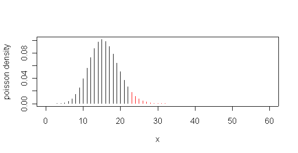
The graph isn't required, but it helps me understand the problem.
Let X be the number of cardiac deaths in a day, and assume that X is Poisson distributed. If the mean of X were really 15.6 per day, then P(X=51) = 7.65e-13 which is almost impossible, but more importantly, P(X>=51) = 1.1e-12 which is also almost impossible, indicating that the observed X = 51 is much too high to have happened by chance if the mean is 15.6.
By inspecting the cumulative distribution in the range 20 to 25, or by using the Poisson quantile function, we find that the probability of observing 23 or more deaths when the mean is 15.6 is very close to 5%, so 23 would be the 5% critical value; any value of X.< 23 or <= 22 would be consistent with a mean of 15.6.
> plot(0:60,dpois(0:60,15.6),type="h",xlab="x",ylab="poisson density")
> dpois(51,15.6)
[1] 7.650953e-13
> 1-ppois(50,15.6)
[1] 1.089351e-12
> ppois(20:25,15.6)
[1] 0.8894101 0.9267591 0.9532429 0.9712058 0.9828818 0.9901675
> qpois(.95,15.6)
[1] 22
> points(23:60,dpois(23:60,15.6),type="h",col="red")
There are 41 twin pairs; to show the femoral neck differences and count the number of negative differences and the number of non-zero differences, use
> dif <- boneden$fn2-boneden$fn1
> dif
[1] -0.04 -0.10 0.01 0.05 -0.16 -0.06 -0.05 -0.07 0.12 -0.03 0.04 -0.09
[13] 0.01 -0.04 -0.03 0.05 0.06 -0.03 0.05 -0.05 0.06 -0.15 0.20 -0.15
[25] 0.11 0.00 0.00 0.25 -0.01 -0.16 -0.02 0.10 -0.04 -0.06 0.07 0.04
[37] -0.05 -0.03 0.14 0.12 -0.09
> length(dif)
[1] 41
> sum(dif<0)
[1] 22
> sum(dif!=0)
[1] 39
Ignore the two pairs with zero differences as they are not informative. If there were no difference between the heavier smoking twin and the lighter smoking twin, the number of negative differences would be Bin(39, 0.5), in which case the probability of getting 22 or more negative differences would be
> 1-pbinom(21,39,0.5)
[1] 0.2611987
which is much greater than 5%. Since what was observed would be very likely under the hypothesis, there is no evidence from the data that the heavier smoking twin tends to have a lighter femoral neck bone density.
We can order the twins in ascending order according to their pack-year differences, then take femoral neck differences of the 20 twins with the highest pack-year differences and find that 15 of the 20 femoral neck differences are negative and none are zero.
> sum(dif[order(boneden$pyr2-boneden$pyr1)[22:41]]<0)
[1] 15
> sum(dif[order(boneden$pyr2-boneden$pyr1)[22:41]]!=0)
[1] 20
> 1-pbinom(14,20,0.5)
[1] 0.02069473
When we consider only the 20 twins with the biggest pack-year differences, the probability of getting 15 or more negative femoral neck differences out of 20 under the hypothesis of indifference is 2.1% which is less than 5% and hence indicates a significant reduction in femoral neck bone density in heavy smokers.
Since FEV in a non-smoking man is N(4.0, 0.5^2), the probability that it is less than 2.5 L and hence he shows functional impairment is 0.0013.
> pnorm(2.5, 4.0, 0.5)
[1] 0.001349898
Similarly, FEV in a smoking man is N(3.5, 0.6^2), so the probability that he shows functional impairment is 0.0478.
> pnorm(2.5, 3.5, 0.6)
[1] 0.04779035
Given an FEV of exactly 4.0 at age 45 his FEV 30 years later, at age 75, will be N(4-0.3(30), (0.2(30))^2), so the probability that he will show functional impairment is 0.894.
> pnorm(2.5, 4.0-0.3*30, 0.2*30)
[1] 0.8943502
Given an FEV of exactly 4.0 at age 25 his FEV 50 years later, at age 75, will be N(4-0.3(50), (0.2(50))^2), so the probability that he will show functional impairment is 0.911.
> pnorm(2.5, 4.0-0.3*50, 0.2*50)
[1] 0.911492
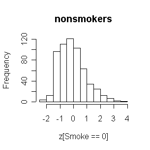
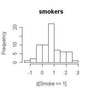
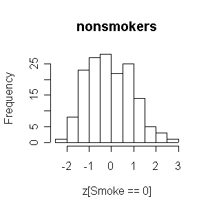
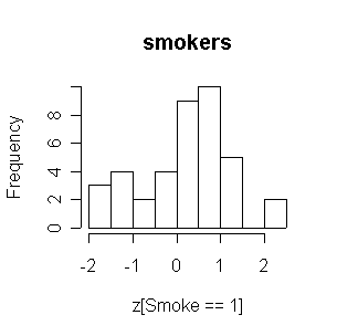
FEV in nonsmokers is positively skewed, and the smokers have generally higher FEVs than nonsmokers.
 |
 |
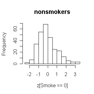
Now the two distributions of FEV are very similar to each other. Both are reasonably normal in shape.
 |
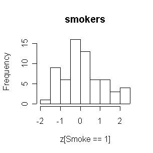 |
The smokers tend to have higher FEVs than the nonsmokers.
 |
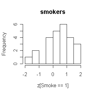 |
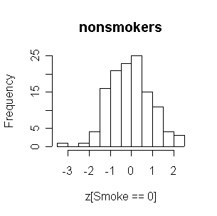
Considering the relatively small number of smokers, the two distributions are comparable. Both are reasonably normal in shape.
 |
 |
> attach(FEV)
> z <- (fev-mean(fev))/sqrt(var(fev))
> hist(z[Smoke==0],main="nonsmokers")
> hist(z[Smoke==1],main="smokers")
> FEV1<-FEV[FEV$Age>=10,]
> detach(FEV)
> attach(FEV1)
> z <- (fev-mean(fev))/sqrt(var(fev))
> hist(z[Smoke==0],main="nonsmokers")
> hist(z[Smoke==1],main="smokers")
> detach(FEV1)
> FEV2<-FEV[FEV$Age>=10&FEV$Sex=="Males",]
> attach(FEV2)
> z <- (fev-mean(fev))/sqrt(var(fev))
> hist(z[Smoke==0],main="nonsmokers")
> hist(z[Smoke==1],main="smokers")
> detach(FEV2)
> FEV3<-FEV[FEV$Age>=10&FEV$Sex=="Females",]
> attach(FEV3)
> z <- (fev-mean(fev))/sqrt(var(fev))
> hist(z[Smoke==0],main="nonsmokers")
> hist(z[Smoke==1],main="smokers")
Suppose that n = 9 observations X1, ..., X9 each have the same variance s2 but are autocorrelated, with
Cor(Xi, Xj) = rij = r|j - i|
for some 0 < r < 1. Apply Equation 5.13 on page 138 to find the standard error of the sample mean. Show that the standard error increases from s /sqrt(n) to s as r increases from 0 to 1. What is the importance of this result for measurements replicated under laboratory conditions?
Simply substitute into Equation 5.13 the values n = 9;ci = 1/9, si = s for all i; and rij = r |j-i| for all i, j, to get
Var(Xbar) = (s2/9){1 + (2/9)[ 8 r + 7 r2 + 6 r3 + 5 r4 + 4 r5+ 3 r6 + 2 r7 + 1 r8 ]
Substituting r = 0 gives Var(Xbar) = s2/9, while substituting r = 1 gives Var(Xbar) = s2. Differentiating Var(Xbar) with respect to r gives a polynomial in r with positive coefficients; since r > 0, the derivative is always positive so Var(Xbar) increases monotonically from s2/9 to s2 as s2 goes from 0 to 1.
When measurements are repeated under laboratory conditions, clean and careful work and reliable equipment will help to ensure that they are independent. If the work is not carefully done, the most common result is positive autocorrelation and this will increase Var(Xbar) so our estimate of the mean will be less reliable.
Suppose that apples from a certain orchard have a mean weight of 90 g with a 10% coefficient of variation. If they are packed 12 to a bag, what is the probability that the bag will weigh less than 1 kg? Given 100 bags, what is the probability that at least 1 will weigh less than 1 kg? Given 1000 bags, what is the probability that at least 10 will weigh less than 1 kg? State any assumptions you make.
Let Y be the total weight of 12 apples and assume that they are chosen randomly and independently. Then E(Y) = 12(90) = 1080 g and Var(Y) = 12(0.1(90))^2 = 972. By the Central Limit Theorem, Y is at least approximately normal; hence Y ~ AN(1080, 972).
P(Y<1000) = F((1000-1080)/sqrt(972)) = 0.00514
> pnorm(1000,1080,sqrt(972))
[1] 0.005143924
Let W be the number of bags out of 100 that weigh less than 1 kg; W ~ Bin(100, 0.005143924), so we can use either the exact binomial or the Poisson approximation:
> 1-pbinom(0,100,pnorm(1000,1080,sqrt(972)))
[1] 0.4029294
> 1-ppois(0,100*pnorm(1000,1080,sqrt(972)))
[1] 0.4021362
Note that these probabilities are easily computed on a calculator.
Now let V be the number of bags out of 1000 that weigh less than 1 kg; V ~ Bin(1000, 0.005143924), so we can use either the exact Binomial or the Poisson approximation to get P(V>=10) = 0.037
> 1-pbinom(9,1000,pnorm(1000,1080,sqrt(972)))
[1] 0.03695049
> 1-ppois(9,1000*pnorm(1000,1080,sqrt(972)))
[1] 0.03735292
or the Normal approximation to either the binomial or the Poisson:
> p <- pnorm(1000,1080,sqrt(972))
> 1-pnorm(9.5,1000*p,sqrt(1000*p*(1-p)))
[1] 0.02707661
> 1-pnorm(9.5,1000*p,sqrt(1000*p))
[1] 0.02738793
The normal approximation isn't very good here because p is so small, but if you are in a hurry and don't have a computer it is the only simple way to do the calculation.
These are grouped data with 287 observations; we need the sample mean and variance. Calculating by hand, use the grouped data formulas; in R, use rep() to ungroup the data and then use the usual functions.
The normal-theory 95% confidence intervals for the mean are (5.017, 5.456) using normal qualtiles, or (5.016, 5.457) using t quantiles. The chi-square confidence interval for the variance is (3.08, 4.27).
Assuming a N(5.237, 1.897) distribution for latency time gives the probability of a latency of at least 8 years as 0.0727.
Not assuming normality, we note that 18+11+4 = 33 out of 287 subjects had latency times of 8 or more years, so p = 0.115 with a 95% confidence interval (based on the normal approximation to the binomial) of (0.078, 0.152).
> onset <- rep(0:10,c(2,6,9,33,49,66,52,37,18,11,4))
> non <- length(onset)
> non
[1] 287
> mean(onset)
[1] 5.236934
> sqrt(var(onset))
[1] 1.897632
> mean(onset)+c(-1,1)*qnorm(.975)*sqrt(var(onset)/non)
[1] 5.017391 5.456477
> mean(onset)+c(-1,1)*qt(.975,non-1)*sqrt(var(onset)/non)
[1] 5.016458 5.457410
> var(onset)*(non-1)/c(qchisq(.975,non-1),qchisq(.025,non-1))
[1] 3.076681 4.272571
> 1-pnorm(8,mean(onset),sqrt(var(onset)))
[1] 0.07268805
> p <- (18+11+4)/non
> p
[1] 0.1149826
> p+c(-1,1)*qnorm(.975)*sqrt(p*(1-p)/non)
[1] 0.0780764 0.1518888
Nifed makes a significant positive difference in heart rate, either comparing level 3 to baseline or comparing the average of the three levels to baseline. Propanolol does not make a significant difference. Neither treatment affects systolic blood pressure significantly (all confidence intervals include 0). The outlier in propanolol is a concern.
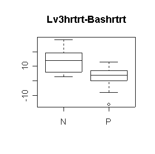
N: mean diff = 13.57, 95% CI = (4.96, 22.18) |
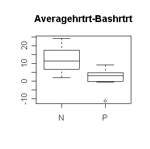
N: mean diff = 12.11, 95% CI = (3.66, 20.56) |

N: mean diff = -5.125, 95% CI = (-30.04, 19.79) |
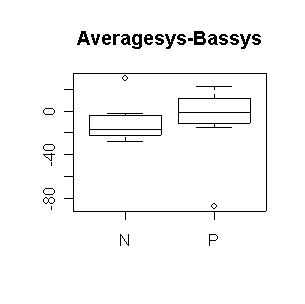
N: mean diff = -9.76, 95% CI = (-28.00, 8.48) |
> boxplot(Lv3hrtrt-Bashrtrt~Trtgrp,data=nifed)
> title("Lv3hrtrt-Bashrtrt")
> boxplot(Lv3sys-Bassys~Trtgrp,data=nifed)
> title("Lv3sys-Bassys")
> boxplot((Lv1hrtrt+Lv2hrtrt+Lv3hrtrt)/3-Bashrtrt~Trtgrp,data=nifed)
> title("Averagehrtrt-Bashrtrt")
> boxplot((Lv1sys+Lv2sys+Lv3sys)/3-Bassys~Trtgrp,data=nifed)
> title("Averagesys-Bassys")
> dif <- (nifed$Lv3hrtrt-nifed$Bashrtrt)[nifed$Trtgrp=="N"]
> mean(dif,na.rm=T)
[1] 13.57143
> n <- sum(!is.na(dif))
> n
[1] 7
> mean(dif,na.rm=T)+c(-1,1)*qt(.975,n-1)*sqrt(var(dif,na.rm=T)/n)
[1] 4.963949 22.178908
> dif <- (nifed$Lv3hrtrt-nifed$Bashrtrt)[nifed$Trtgrp=="P"]
> mean(dif,na.rm=T)
[1] 1.333333
> n <- sum(!is.na(dif))
> n
[1] 9
> mean(dif,na.rm=T)+c(-1,1)*qt(.975,n-1)*sqrt(var(dif,na.rm=T)/n)
[1] -5.422642 8.089309
> dif <- (nifed$Lv3sys-nifed$Bassys)[nifed$Trtgrp=="N"]
> mean(dif,na.rm=T)
[1] -5.125
> n <- sum(!is.na(dif))
> n
[1] 8
> mean(dif,na.rm=T)+c(-1,1)*qt(.975,n-1)*sqrt(var(dif,na.rm=T)/n)
[1] -30.04362 19.79362
> dif <- (nifed$Lv3sys-nifed$Bassys)[nifed$Trtgrp=="P"]
> mean(dif,na.rm=T)
[1] -5
> n <- sum(!is.na(dif))
> n
[1] 8
> mean(dif,na.rm=T)+c(-1,1)*qt(.975,n-1)*sqrt(var(dif,na.rm=T)/n)
[1] -31.58794 21.58794
> dif <- ((nifed$Lv1hrtrt+nifed$Lv2hrtrt+nifed$Lv3hrtrt)/3-nifed$Bashrtrt)[nifed$Trtgrp=="N"]
> mean(dif,na.rm=T)
[1] 12.11111
> n <- sum(!is.na(dif))
> n
[1] 6
> mean(dif,na.rm=T)+c(-1,1)*qt(.975,n-1)*sqrt(var(dif,na.rm=T)/n)
[1] 3.664283 20.557939
> dif <- ((nifed$Lv1hrtrt+nifed$Lv2hrtrt+nifed$Lv3hrtrt)/3-nifed$Bashrtrt)[nifed$Trtgrp=="P"]
> mean(dif,na.rm=T)
[1] 1.541667
> n <- sum(!is.na(dif))
> n
[1] 8
> mean(dif,na.rm=T)+c(-1,1)*qt(.975,n-1)*sqrt(var(dif,na.rm=T)/n)
[1] -3.483160 6.566493
> dif <- ((nifed$Lv1sys+nifed$Lv2sys+nifed$Lv3sys)/3-nifed$Bassys)[nifed$Trtgrp=="N"]
> mean(dif,na.rm=T)
[1] -9.761905
> n <- sum(!is.na(dif))
> n
[1] 7
> mean(dif,na.rm=T)+c(-1,1)*qt(.975,n-1)*sqrt(var(dif,na.rm=T)/n)
[1] -28.004202 8.480393
> dif <- ((nifed$Lv1sys+nifed$Lv2sys+nifed$Lv3sys)/3-nifed$Bassys)[nifed$Trtgrp=="P"]
> mean(dif,na.rm=T)
[1] -9.428571
> n <- sum(!is.na(dif))
> n
[1] 7
> mean(dif,na.rm=T)+c(-1,1)*qt(.975,n-1)*sqrt(var(dif,na.rm=T)/n)
[1] -43.40758 24.55043
Taking differences in femoral shaft bone density, we find the 95% confidence interval for the mean difference to be (-0.067, 0.005) which includes 0, indicating that there is no evidence of a difference in femoral shaft bone density between the lighter and heavier smoker.
> dif <- boneden$fs2-boneden$fs1
> dif
[1] 0.04 0.12 -0.19 -0.09 -0.18 -0.07 0.07 -0.01 0.08 -0.06 -0.03 -0.12
[13] 0.08 -0.14 0.11 -0.10 0.05 0.14 0.03 -0.14 0.01 0.10 0.10 -0.16
[25] 0.05 -0.06 -0.04 0.04 -0.42 -0.17 -0.03 0.10 -0.10 -0.08 -0.03 -0.04
[37] 0.10 -0.20 -0.03 -0.04 0.06
> mean(dif)
[1] -0.03048780
> mean(dif)+c(-1,1)*qt(.975,40)*sqrt(var(dif)/41)
[1] -0.066703514 0.005727904
Even when we look only at the 20 twin pairs with the greatest pack-year differences, the 95% confidence interval (-0.128, 0.004) includes zero, again indicating that there is no evidence of a difference in femoral shaft bone density between the lighter and heavier smoker.
> difh <- dif[order(boneden$pyr2-boneden$pyr1)[22:41]]
> mean(difh)
[1] -0.062
> mean(difh)+c(-1,1)*qt(.975,19)*sqrt(var(difh)/20)
[1] -0.127760867 0.003760867
[Interesting but not required] If we continue from (C) with the femoral neck differences, we find the 95% confidence interval for the mean to be (-0.030, 0.029) which includes 0, indicating that there is no evidence of a difference in femoral neck bone density between the lighter and heavier smoker.
> mean(dif)
[1] -0.0007317073
> mean(dif)+c(-1,1)*qt(.975,40)*sqrt(var(dif)/41)
[1] -0.03012505 0.02866164
However, when we look only at the 20 twin pairs with the greatest pack-year differences, the 95% confidence interval (-0.074, -0.001) is entirely negative, indicating a significantly lower bone density in the heavier smoking twin.
> difh <- dif[order(boneden$pyr2-boneden$pyr1)[22:41]]
> mean(difh)
[1] -0.0375
> mean(difh)+c(-1,1)*qt(.975,19)*sqrt(var(difh)/20)
[1] -0.074127921 -0.000872079