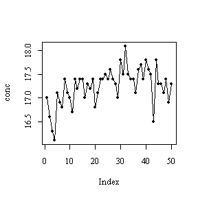

There isn't much you can say about the shape of a distribution with only 50 observations, but the stem and leaf plot indicates a more or less bell-shaped distribution.
  The decimal point is 1 digit(s) to the left of the |

  160 | 0
  162 | 0
  164 | 0
  166 | 00
  168 | 0000
  170 | 000000000
  172 | 0000000
  174 | 00000000000000000
  176 | 0000
  178 | 000
  180 | 0
The time sequence plot is also inconclusive with only 50 points, but does seem to rise, at least for the first 30 steps (60 hours), indicating a trend, and have a cycle of about 10 steps (20 hours).
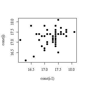
The lag-1 scatterplot (plotting the concentration at step i on the Y-axis against concentration at the previous step i-1 on the X-axis) shows only an unoriented scatter of points, suggesting that there is no lag-1 autocorrelation in this time series.
|
|
|
Sample range: 5.2 - 2 = 3.2
Sample variance: s2 = 0.8663
Sample standard deviation: s = 0.9308
All of these measures of dispersion are unaffected if we subtract 1, or any other constant, from each observation.
The box plot in original units is skewed to the right (has a long upper tail) because the data span several orders of magnitude. A log transformation makes the distribution much more symmetric.
|
|
|
The set-up described here for the number of defectives in a lot matches the assumptions of the Bin(100, 0.1) distribution. Note that while 10 is the most probable value, any outcome between 5 and 15 is reasonably likely; I have replotted for x = 0 to 20 to show this (not required).
|
|
|
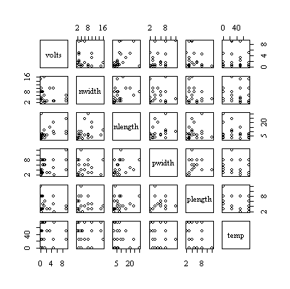
The scatterplot matrix does not reveal any strong pairwise relationships. None of the histograms suggest normal distributions. It appears that the study is at least partly experimental; e.g. temperature was set to four different values by the design of the study. The other variables do not seem to follow any such regular pattern and may have been observed, not controlled.

|
|
|
|
|
|
|
|
|
Firing at 125 `F gives brick densities that are usually lower than those from the other temperatures studied.
|
|
|
The series isn't long enough to reveal any trend.
The lag-1 scatterplot shows no evidence of autocorrelation.
|
|
|