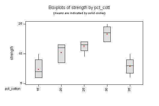
(Note that for exam purposes, a comparative dot plot would be better than a comparative box plot.)
One-way Analysis of Variance

Analysis of Variance for strength
Source     DF        SS        MS        F        P
pct_cott    4    475.76    118.94    14.76    0.000
Error      20    161.20      8.06
Total      24    636.96
                                   Individual 95% CIs For Mean
                                   Based on Pooled StDev
Level       N      Mean     StDev  ------+---------+---------+---------+
15          5     9.800     3.347  (-----*----)
20          5    15.400     3.130              (----*----)
25          5    17.600     2.074                  (----*----)
30          5    21.600     2.608                          (----*----)
35          5    10.800     2.864    (-----*----)
                                   ------+---------+---------+---------+
Pooled StDev =    2.839               10.0      15.0      20.0      25.0

95% Confidence interval for s2: (4.72, 16.8)
Conclusions:
There is strong evidence (P < 0.001) that % cotton affects the mean strength. The highest mean strength was at 30% cotton. Further trials around 30% cotton may help find the % cotton that gives the highest strength.
Assumptions:
Independent observations; variation in strength follows a normal distribution with the same variance at each level of % cotton.
Regression Analysis

The regression equation is
strength = 10.9 + 0.164 pct_cotton

Predictor        Coef       StDev          T        P
Constant       10.940       3.764       2.91    0.008
pct_cott       0.1640      0.1449       1.13    0.269

S = 5.122       R-Sq = 5.3%      R-Sq(adj) = 1.2%

Analysis of Variance

Source            DF          SS          MS         F        P
Regression         1       33.62       33.62      1.28    0.269
Residual Error    23      603.34       26.23
  Lack of Fit      3      442.14      147.38     18.29    0.000
  Pure Error      20      161.20        8.06
Total             24      636.96

Unusual Observations
Obs   pct_cott   strength         Fit   StDev Fit    Residual    St Resid
 21       35.0       7.00       16.68        1.77       -9.68       -2.01R

R denotes an observation with a large standardized residual
Conclusions:
There is strong evidence (P < 0.001) that the relationship between strength and % cotton is not linear over the range of % cotton studied. We could try fitting a quadratic relationship (but that won't be on the exam). Since the relationship is not linear the slope of the fitted line has no meaning, so we do not test the slope. Note that the nonlinearity is obvious just by looking at the graph.
Assumptions:
Independent observations; variation in strength follows a normal distribution with the same variance at each level of % cotton.
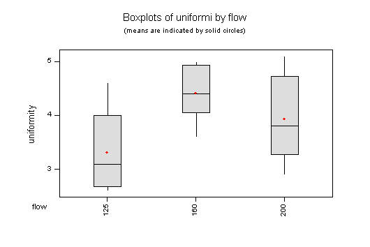
(Note that for exam purposes, a comparative dot plot would be better than a comparative box plot.)
One-way Analysis of Variance

Analysis of Variance for uniformi
Source     DF        SS        MS        F        P
flow        2     3.648     1.824     3.59    0.053
Error      15     7.630     0.509
Total      17    11.278
                                   Individual 95% CIs For Mean
                                   Based on Pooled StDev
Level       N      Mean     StDev  --+---------+---------+---------+----
125         6    3.3167    0.7600   (-------*--------)
160         6    4.4167    0.5231                  (--------*--------)
200         6    3.9333    0.8214           (--------*--------)
                                   --+---------+---------+---------+----
Pooled StDev =   0.7132            2.80      3.50      4.20      4.90

95% Confidence interval for s2: (0.278, 1.22)
Conclusions:
There is some evidence (P = 0.053) that C2F6 flow affects the mean uniformity. Note that the result is not, strictly speaking, significant by a test at the 5% level but it is very close to 5%. A 5% test would accept the hypothesis of no difference due to C2F6 flow.
Assumptions:
Independent observations; variation in compressive strength follows a normal distribution with the same variance at each level of C2F6 flow.
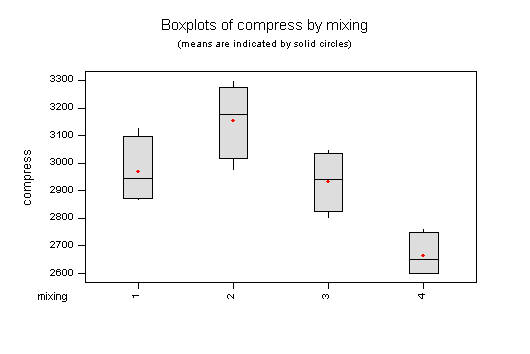
(Note that for exam purposes, a comparative dot plot would be better than a comparative box plot.)
One-way Analysis of Variance

Analysis of Variance for compress
Source     DF        SS        MS        F        P
mixing      3    489740    163247    12.73    0.000
Error      12    153908     12826
Total      15    643648
                                   Individual 95% CIs For Mean
                                   Based on Pooled StDev
Level       N      Mean     StDev  ---+---------+---------+---------+---
1           4    2971.0     120.6                 (------*-----)
2           4    3156.3     136.0                           (-----*-----)
3           4    2933.8     108.3                (-----*-----)
4           4    2666.3      81.0  (-----*-----)
                                   ---+---------+---------+---------+---
Pooled StDev =    113.3            2600      2800      3000      3200

95% Confidence interval for s2: (6595, 34949)
Conclusions:
There is strong evidence (P < 0.001) that mixing technique affects the compressive strength of concrete. Mixing technique 4 gave a lower mean compressive strength than the others.
Assumptions:
Independent observations; variation in compressive strength follows a normal distribution with the same variance under each mixing technique.
Two-way Analysis of Variance

Analysis of Variance for life
Source        DF        SS        MS        F        P
material       2     10684      5342     7.91    0.002
temp           2     39119     19559    28.97    0.000
Interaction    4      9614      2403     3.56    0.019
Error         27     18231       675
Total         35     77647

95% Confidence interval for s2: (422, 1251)
Conclusions:
There is some evidence (P = 0.019) that battery material and ambient temperature interact; that is, they both affect battery life but the effect of ambient temperature is different with different materials. Even if we ignore the interaction, there is strong evidence that ambient temperature (P < 0.001) and battery material (P = 0.002) separately affect battery life.
Assumptions:
Independent observations; variation in battery life follows a normal distribution with the same variance at each combination of battery material and ambient temperature.
Two-way Analysis of Variance

Analysis of Variance for finish
Source        DF        SS        MS        F        P
paint          1       356       356     1.90    0.193
dry_time       2        27        14     0.07    0.930
Interaction    2      1879       939     5.03    0.026
Error         12      2243       187
Total         17      4504

95% Confidence interval for s2: (96.1, 509)
Conclusions:
There is some evidence (P = 0.026) that paint type and dry time interact; that is, they both affect finish but the effect of paint type is different with different dry times. If we were to ignore the interaction, we would say that there is no evidence that dry time (P = 0.930) or paint type (P = 0.193) affect finish, but this conclusion would be misleading.
Assumptions:
Independent observations; variation in finish follows a normal distribution with the same variance at each combination of paint type and dry time.
Two-way Analysis of Variance

Analysis of Variance for current
Source        DF        SS        MS        F        P
glass          1   14450.0   14450.0   273.79    0.000
phosphor       2     933.3     466.7     8.84    0.004
Interaction    2     133.3      66.7     1.26    0.318
Error         12     633.3      52.8
Total         17   16150.0

95% Confidence interval for s2: (27.1, 144)
Conclusions:
There is no evidence (P = 0.318) that glass type and phosphor type interact, so we can proceed to test the main effects. There is strong evidence that phosphor type (P = 0.004) and glass type (P < 0.001) both affect brightness, and the effect of either one does not depend on the other.
Assumptions:
Independent observations; variation in brightness follows a normal distribution with the same variance at each combination of glass type and phosphor type.