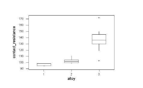
The alloys give different contact resistance with almost no overlap in their distributions. Alloy 1 gives the lowest contact resistance and is the least variable and alloy 3 gives the highest and is the most variable.
Since the contacts of a relay must conduct electricity, lower contact resistance is better than higher, so alloy 1 would be the best for the purpose and alloy 2 would be almost as good. The lower variability of alloy 1 would also be advantageous, giving more consistent performance.
Q2
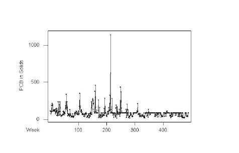
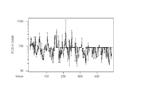
The time sequence plot shows annual cycles peaking in the late spring and occasional extreme high values. There is also an indication that high values may have been truncated; in the second half of the series few values exceed 89 and many are exactly 89, and this shows as a horizontal band on the plot. There is a similar but less pronounced effect in the first half, suggesting that in the first four years a few high values were truncated at 77. Because of the truncation, it is hard to say whether or not there is any trend. We would hope that the level of PCB is decreasing over time but we can't see that here because of the truncation.
Plotting on a log scale makes the annual cycles and the truncation of high values a bit more evident. It emphasizes the variation at low levels of PCB while reducing the visual impact of the high values. The very low values may not be of interest, however, if they are in the "environmentally safe" range, but we don't know what that range is. The truncation of high values makes it impossible to tell if there is a downward trend.
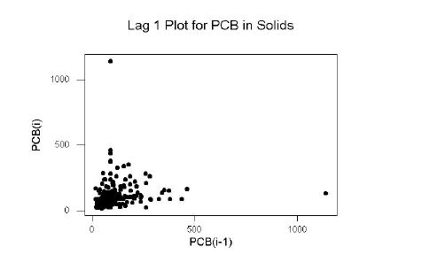
The Lag-1 plot is uninterpretable on the linear scale. Note that the one extreme high point in the time sequence plot shows up as two outliers on the Lag-1 plot.
On a log scale, the Lag-1 plot shows positive autocorrelation. Note that the values truncated at 89 show as horizontal and vertical bands in this plot.
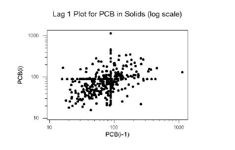
The log transformation makes it easier to see the cycles, truncation and autocorrelation, but may not be useful if only the high PCB levels are of interest.
[You might be interested to see the Case Study on Niagara River Pollution from which this series is taken.]
Q3
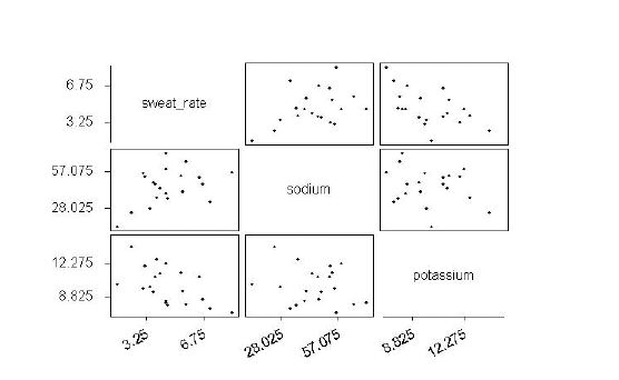
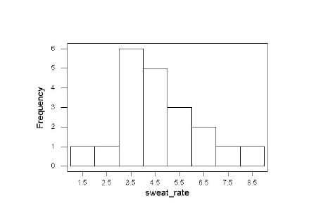
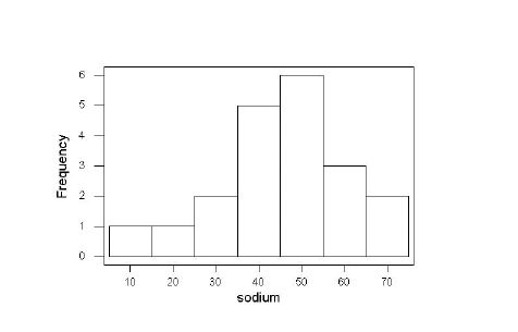
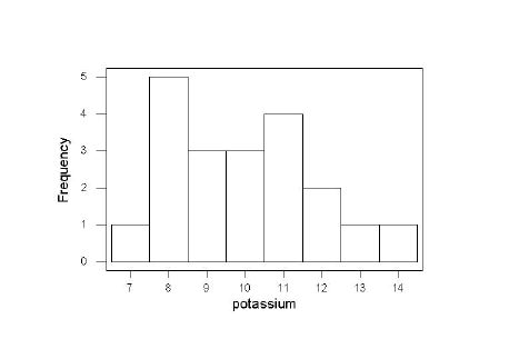
The scatterplot matrix is not convincing because the sample is so small, but there is a suggestion that sweat rate is negatively correlated with sodium and negatively correlated with potassium, while sodium and potassium do not appear to be correlated with each other. Again, it is hard to assess normality from a small sample, but the histograms for all three variables are more or less bell-shaped. The histograms are not quite symmetric, but that could easily happen by chance in a small sample.
Q4
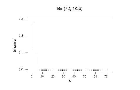
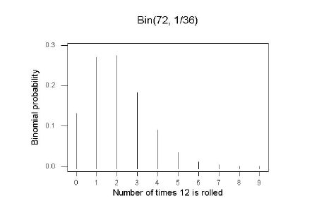
There are 36 equally-likely ways that two independent fair 6-sided dice can roll and only one of these (two sixes) gives a twelve, so the probability of getting a twelve is 1/36. Alternatively, the probability of getting a six on one die is 1/6 so the probability of getting sixes on two independent dice is (1/6)^2 = 1/36.
With 72 independent rolls of two independent dice, the chance of a twelve being 1/36 on each roll, the total number of twelves obtained will follow a Binomial distribution with n = 72 and p = 1/36. The following graphs were plotted in Minitab.