Solutions last corrected 2001-11-01 07:30
I have used R to prepare these solutions; you may use any software you like. I recommend that you do these problems on your calculator whenever possible and then use R to verify your results. Then you get to see the calculations both ways.
Full marks = 85
Suppose that average weight of men is 70 kg and the standard deviation is 10 kg, while for women the average is 60 kg and the standard deviation is 8 kg. If 10 men and 6 women get on an elevator, what is the probability that their combined weight will exceed 1 tonne? Will exceed 1.1 tonnes? State any additional assumptions you make.
Let Y be the total weight; it is the sum of the weights of 10 men (mean = 70 kg, standard deviation = 10 kg) and 6 women (mean = 60 kg, standard deviation = 8 kg). Assuming independence, the variances add. Assuming approximate normality of weight, the central limit theorem says that the distribution of the total weight will be closer to a normal distribution than is the distribution of the individual weights.
E[Y] = 10 * 70 + 6 * 60 = 1060 kg
Var[Y] = 10 * 102 + 6 * 82 = 1384
P(Y >= 1000) = 1 - F((1000 - 1060) / sqrt(1384)) = 1 - F( -1.61281) = 0.9466071 = 0.947
P(Y >= 1100) = 1 - F((1100 - 1060) / sqrt(1384)) = 1 - F( 1.075207 ) = 0.1411411 = 0.141
> meanwt <- 10*70 + 6*60
> varwt <- 10*10^2 + 6*8^2
> 1-pnorm((1000-meanwt)/sqrt(varwt))
[1] 0.9466071
> 1-pnorm((1100-meanwt)/sqrt(varwt))
[1] 0.1411411
Suppose that reportable accidents at a round-the-clock construction site occur independently of each other at an average rate of 0.1 accidents per day. Compute the probabilities of the following events: (a) no accidents in November; (b) more than four accidents in November; (c) no accidents next week; (d) five or more accident-free weeks over the next ten weeks; (e) seven or more accident-free weeks over the next ten weeks; (f) no accidents in the next seven weeks; (g) the time between accidents exceeds seven weeks. State any additional assumptions you make.
Assume that the accidents follow a Poisson Process; that is, they occur randomly, one at a time, independently of each other, at a constant average rate of 0.1 per day.
(a) Let Y be the number of accidents in November; E[Y] = 30 * 0.1 = 3, so Y ~ Pois(3). Compute P(Y = 0).
> dpois(0,3)
[1] 0.04978707
(b) Compute P(Y > 4) = 1 - P(Y <= 3)
> 1 - ppois(3,3)
[1] 0.3527681
(c) Let X be the number of accidents in a week; as in (a), we find that X ~ Pois(0.7). Compute p = P(X = 0).
> dpois(0,.7)
[1] 0.4965853
(d) Let W be the number of accident-free weeks over the next 10 weeks; W ~ Bin(10, p) where p was calculated in (c). Compute P(W >= 5) = 1 - P(W <= 4).
> 1 - pbinom(4, 10, dpois(0,.7))
[1] 0.6146154
(e) Compute P(W >= 7) = 1 - P(W <=6)
> 1 - pbinom(6, 10, dpois(0,.7))
[1] 0.1663302
(f) Let V be the number of accidents over the next 7 weeks; V ~ Pois(4.9). Compute P(V = 0). Note that both of the following two calculations are correct.
> dpois(0,4.9)
[1] 0.007446583
> dbinom(7, 7, dpois(0,.7))
[1] 0.007446583
(g) Let T be the time in days to the next accident; since T ~ Exp(1/0.1), we compute P(T > 49) = exp(-0.1*49) = 0.007446583 which is exactly the same answer as we got in (f), because T > 49 if and only if V = 0.
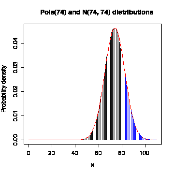
Graph the probability density function for a Poisson distribution with mean = 74. Superimpose a graph of the approximating normal probability density function. Use vertical bars to show the Poison probabilities and use a smooth line in a different colour for the normal curve. Compute the exact Poisson probability of getting 80 or more. Compare the exact calculation with the normal approximation, computed with and without the continuity correction.
> plot(0:110,dpois(0:110,74),type="h",xlab="x",ylab="Probability density",main="Pois(74) and N(74, 74) distributions")
> lines(0:110,dnorm(0:110,74,sqrt(74)),col="red")
> lines(80:110,dpois(80:110,74),type="h",col="blue")
The probability of getting 80 or more is 0.2576 by the exact Poisson calculation, 0.2805 by the normal approximation without continuity correction, and 0.2613 by the normal approximation with continuity correction. The continuity correction improves the approximation.
> 1 - ppois(79,74)
[1] 0.2575723
> 1 - pnorm(79,74,sqrt(74))
[1] 0.2805400
> 1 - pnorm(79.5,74,sqrt(74))
[1] 0.2612937
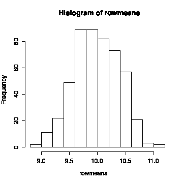
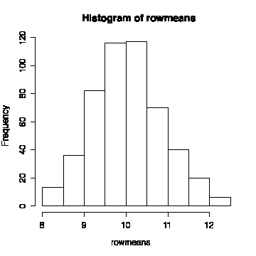
Generate 500 samples, each with n = 25 independent observations from a normal distribution with mean = 10 and standard deviation = 2. Arrange the data in 500 rows, so that each row is one sample. Use these samples to demonstrate the Central Limit Theorem, which says that the distribution of the sample mean will be normal with mean = 10 and standard deviation = 2/5.
Since you are generating your own data, your results will differ a bit from mine, but not by much. The mean of the row means should be very close to 0 and the standard deviation should be very close to 0.4 and the histogram should look normal, as predicted by the central limit theorem.
> inormdata <- matrix(rnorm(500*25,10,2),ncol=25)
> rowmeans <- apply(inormdata,1,mean)
> mean(rowmeans)
[1] 9.981068
> sqrt(var(rowmeans))
[1] 0.3942401
> hist(rowmeans)
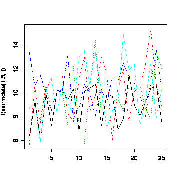
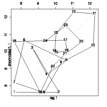
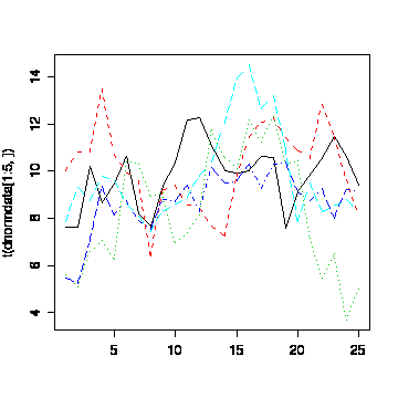
The following graphs are not required, but will help you understand the difference between the samples of independent observations in Question 4 and the samples of dependent data in Question 5. The lag 1 plot of the first row shows a random scatter (no lag-1 autocorrelation) and the sequence plots of the first 5 rows show a random up-and-down variation free of autocorrelation. Note the use of matplot() to plot the columns of a matrix, and t() to transpose the matrix so that the samples are in the columns instead of the rows.We need library(ts) to attach the time series library, where lag.plot() is found.
> library(ts)
> lag.plot(inormdata[1,])
> matplot(t(inormdata[1:5,]),type="l")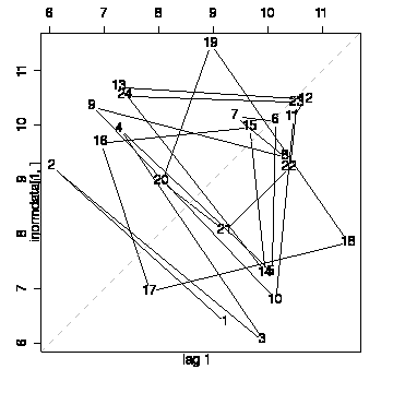
The attached data file gives 500 samples of n = 25 observations from a normal distribution with mean = 10 and standard deviation = 2. The data are arranged in 500 rows, so that each row is one sample. Is the distribution of the sample mean normal with mean = 10 and standard deviation = 2/5? How are these samples different from the samples you generated in Question 4? Use appropriate graphs to explain your answer.
You should get the same numbers here as I got because we are using the same data. Note that read.table() gives a data frame; I converted this to a matrix with as.matrix() because the lag plot wouldn't work for a row of a data frame.
We observe that the standard error of the sample mean is 0.818, which is about twice what the central limit theorem predicts. But the lag plot and the sequence plots show that there is positive autocorrelation: compare them to the plots in Question 4, where we know the data are independent. The points on the lag plot lie more along the diagonal, and the sequence plots tend to stay high or low longer, rather than fluctuate up or down at each step. We know that if the data are positively autocorrelated rather than independent, the standard error of the sample mean will be inflated, and that is what is observed here.
> dnormdata <- as.matrix(read.table("dnormdata.txt"))
> dim(dnormdata)
[1] 500  25
> rowmeans <- apply(dnormdata,1,mean)
> mean(rowmeans)
[1] 10.03812
> sqrt(var(rowmeans))
[1] 0.818167
> hist(rowmeans)
> lag.plot(dnormdata[1,])
> matplot(t(dnormdata[1:5,]),type="l")
4-58 (p 121) [5 marks]
Let X be the number of non-defective components.
(a) Compute P(X >= 100) where X ~ Bin(100, .98)
> 1 - pbinom(99,100,.98)
[1] 0.1326196
(b) Compute P(X >= 100) where X ~ Bin(102, .98)
> 1 - pbinom(99,102,.98)
[1] 0.6657502
(b) Compute P(X >= 100) where X ~ Bin(105, .98)
> 1 - pbinom(99,105,.98)
[1] 0.9807593
4-108 (p 142) [5 marks]
Let X be the number of totes that exceed the moisture content target, out of 30 tested. X ~ Bin(30, p) where p is not given.
We need to find p so that P(X >= 1) = 0.9, or P(X = 0) = 0.1. But P(X = 0) = (1 - p)^30 so the answer is
> 1 - 0.1^(1/30)
[1] 0.07388127
4-110 (p 142) [9 marks]
Let X be the number of flaws in a panel; X ~ Pois(0.02), so the probability that a panel is free of flaws is P(X = 0).
> dpois(0,0.02)
[1] 0.9801987
(a) Let Y be the number of panels without flaws out of 50 tested. Since Y ~ Bin(50, exp(-0.02)) the probability of no flaws in all 50 panels is P(Y = 50) = (e-0.02)50 = e-1 = 0.368.
> dbinom(50,50,dpois(0,0.02))
[1] 0.3678794
(b) Since a proportion 1 - 0.9801987 = 0.01980133 of all panels are flawed, the expected number to test before finding a flawed panel is 1/ 0.01980133 = 50.50167 or 50.5 panels.
(c) Let W be the number of panels with 2 or more flaws out of 50 inspected. Since W ~ Bin(50, P(X >=2)) we must compute P(W <= 2).
> pbinom(2,50,1-ppois(1,0.02))
[1] 0.9999999
5-44 (p 169) [6 marks]
Let X be the line width; we are given that X ~ N(0.5, 0.052).
(a) Here are four different ways to compute P(X > 0.62) in R.
> 1 - pnorm((.62 - .5)/.05,0,1)
[1] 0.008197536
> 1 - pnorm((.62 - .5)/.05)
[1] 0.008197536
> 1 - pnorm(.62,.5,.05)
[1] 0.008197536
> pnorm(.62,.5,.05,lower.tail=F)
[1] 0.008197536
(b) Here are two different ways to compute P(0.47 < X < 0.63) in R.
> pnorm((0.63 - 0.5)/.05) - pnorm((0.47 - 0.5)/.05)
[1] 0.7210857
> pnorm(.63,.5,.05) - pnorm(.47,.5,.05)
[1] 0.7210857
(c) Find q such that P(X < q) = 0.9, i.e. solve for q in F((q - 0.5)/.05) = 0.9. You can interpolate in Table II or you can read the answer directly from Table IV, which gives 1.282 for infinite degrees of freedom at the bottom of the a = 0.1 column. That is, F(1.282) = 0.9 so (q - 0.5)/.05 = 1.282 and hence q = 0.05 * 1.282 + 0.5 = 0.5641. The qnorm() function in R can give the answer directly.
> 0.05*qnorm(0.9) + 0.5
[1] 0.5640776
> qnorm(0.9,0.5,0.05)
[1] 0.5640776
5-130 (p 197) [5 marks]
Let T be the lifetime of an amplifier and let the two types be "A" and "B". We are given that T | A ~ Exp(1/20000) and T | B ~ Exp(1/50000), also that P(A) = 0.1 and P(B) = 0.9. Hence, using Total Probability and the formula for the cumulative distribution function of the exponential distribution, we get
P(T < 60000) = P(T < 60000 | A) * P(A) + P(T < 60000 | B) * P(B)
= ( 1 - e-60000/20000 ) * (0.1) + ( 1 - e-60000/50000 ) * (0.9)
= (1 - e-3) * (0.1) + (1 - e-1.2) * (0.9) = 0.7239
> (1-exp(-3))*0.1+(1-exp(-1.2))*0.9
[1] 0.7239465
> pexp(60000,1/20000)*0.1 + pexp(60000,1/50000)*0.9
[1] 0.7239465