Marks are indicated in red. Full marks = 90.
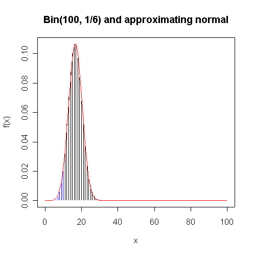
The normal approximation to the Bin(100, 1/6) distribution is very close graphically; the normal approximation to P(X < 10) = 0.0427 is about as good with (0.0490) or without (0.0368) the continuity correction.
> plot(0:100,dbinom(0:100,100,1/6),type="h",xlab="x",ylab="f(x)")
> lines(0:10,dbinom(0:10,100,1/6),type="h",col="blue")
> lines(0:100,dnorm(0:100,100/6,sqrt(100*5/36)),col="red")
> title(main="Bin(100, 1/6) and approximating normal")
> pbinom(10,100,1/6)
[1] 0.04269568
> pnorm(10.5,100/6,sqrt(100*5/36))
[1] 0.04899367
> pnorm(10,100/6,sqrt(100*5/36))
[1] 0.03681914
The normal approximation to the Bin(10, 1/6) distribution is not very close graphically; the normal approximation to P(X < 1) = 0.485 is much better with (0.444) than without (0.286) the continuity correction.
> plot(-3:10,dbinom(-3:10,10,1/6),type="h",xlab="x",ylab="f(x)")
> lines(0:1,dbinom(0:1,10,1/6),type="h",col="blue")
> lines(seq(-3,10,len=50),dnorm(seq(-3,10,len=50),10/6,sqrt(10*5/36)),col="red")
> title(main="Bin(10, 1/6) and approximating normal")
> pbinom(1,10,1/6)
[1] 0.4845167
> pnorm(1.5,10/6,sqrt(10*5/36))
[1] 0.4437685
> pnorm(1,10/6,sqrt(10*5/36))
[1] 0.2858038
> normhist <-
function (x)
{
xgr <- seq(min(x), max(x), len = 50)
hist(x, freq = F, col = "blue")
lines(xgr, dnorm(xgr, mean(x), sqrt(var(x))), col = "red")
invisible()
}
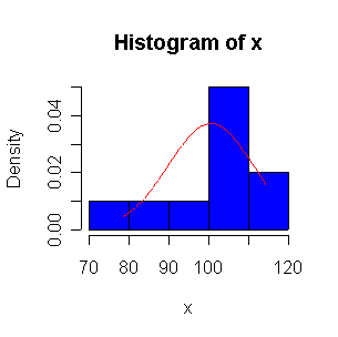
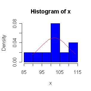
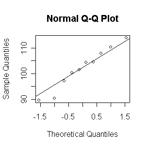
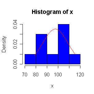
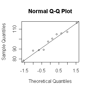
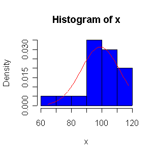
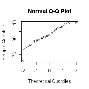
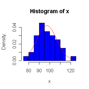
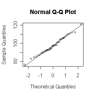
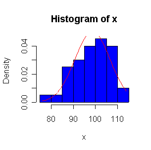
> xx <- rnorm(10,100,10)
> normhist(xx)
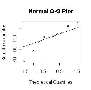
> qqnorm(xx)
> qqline(xx)
 |
 |
 |
 |
 |
 |
 |
 |
 |
 |
 |
 |
 |
 |
 |
 |
 |
 |
 |
 |
 |
 |
 |
 |
 |
 |
 |
 |
 |
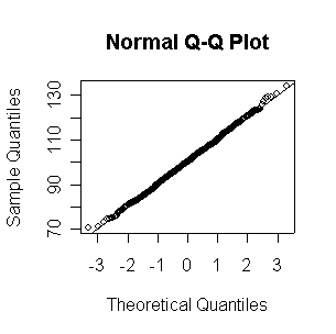 |
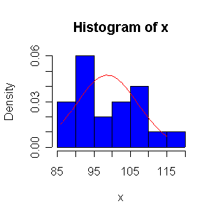
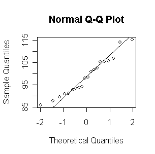
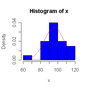
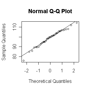
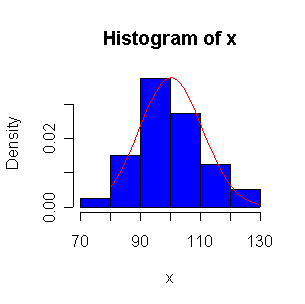
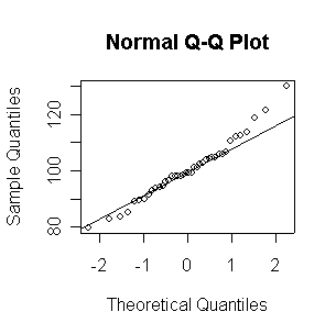
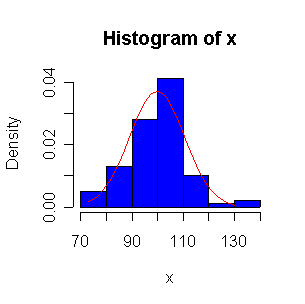
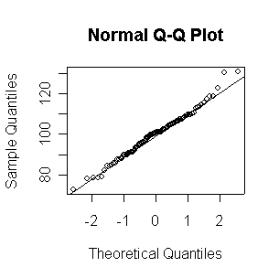
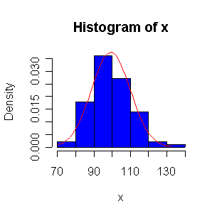
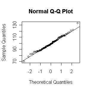
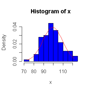
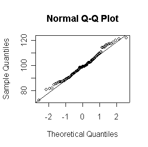
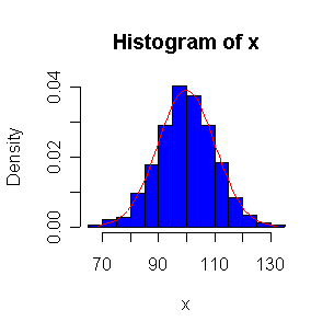
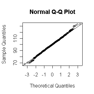
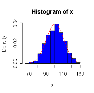
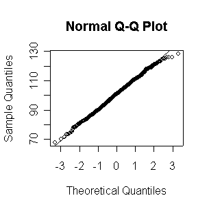
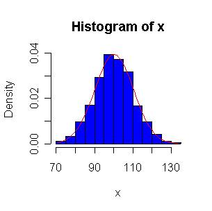
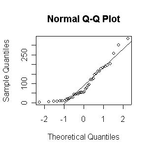
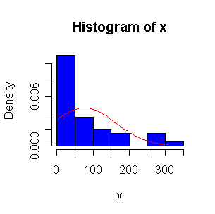
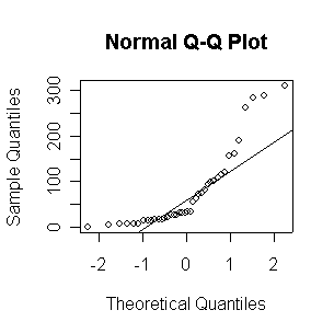
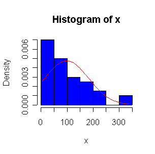
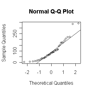
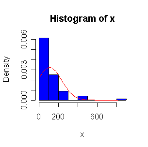
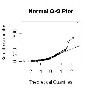
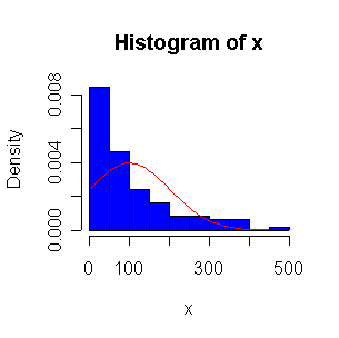
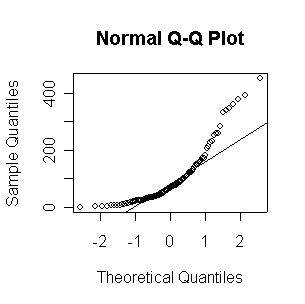
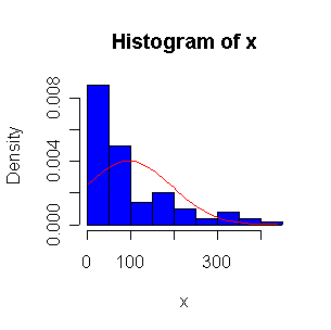
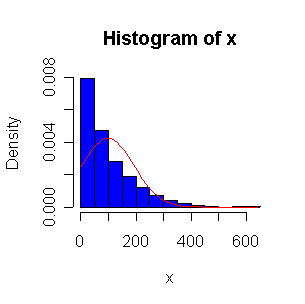
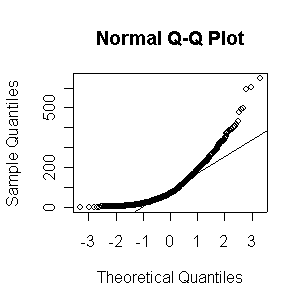
Not until n = 100 does the histogram begin to look Normal, and even then it is usually quite skewed. The QQ plot is reasonably straight when n = 40, except for the tails of the distribution. This suggests that at least 40 observations, but preferably 100 or more, are needed to demonstrate Normality.
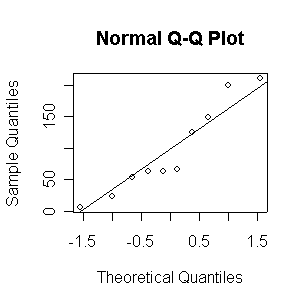
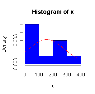
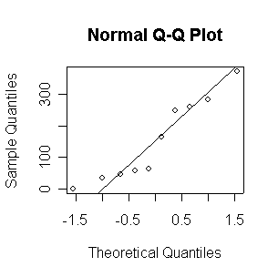
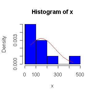
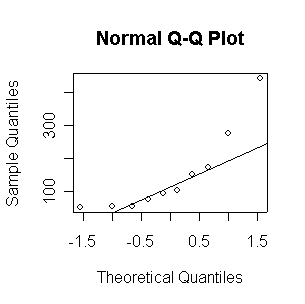
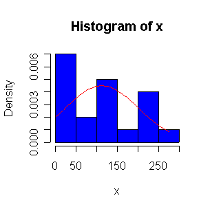
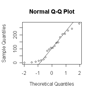
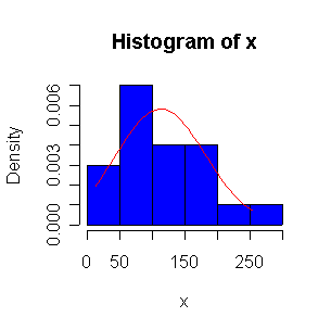
> xx <- rexp(10,1/100)
> normhist(xx)
> qqnorm(xx)
> qqline(xx)
 |
 |
 |
 |
 |
 |
 |
 |
 |
 |
 |
 |
 |
 |
 |
 |
 |
 |
 |
 |
 |
 |
 |
 |
 |
 |
 |
 |
 |
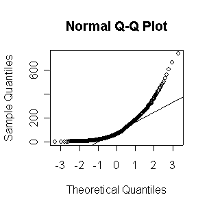 |
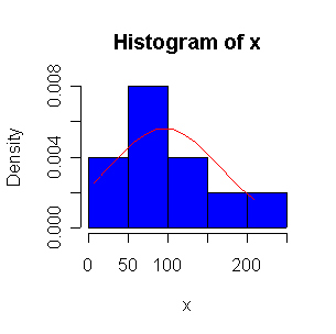
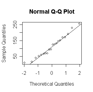
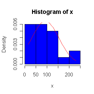
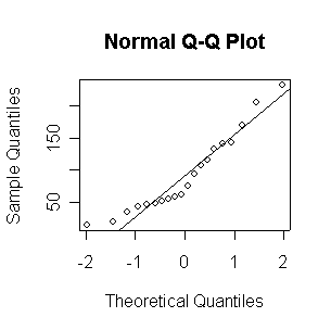
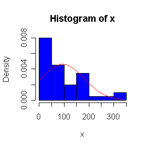
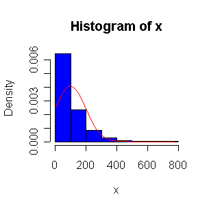
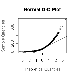
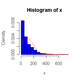
When n = 10 or 20, the histogram will often look as Normal, and the Normal QQ plot will often look as straight, as you would get with a Normal sample of the same size. When n = 40 or more, the histogram is consistently skewed and the Normal QQ plot shows a characteristic curvature that reliably indicates that the data did not come from a Normal distribution.
The Exp(1/100) distribution has mean = standard deviation = 100. The Central Limit Theorem states that if n = 100, the distribution of the sample mean will be approximately Normal with mean = 100 and standard deviation = 100/sqrt(100) = 10.
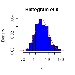
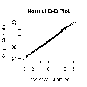
Here we have 500 realizations of the sample mean; the histogram and Normal QQ plot indicate that the sampling distribution is very close to Normal, even though the data came from a non-normal distribution. The observed mean of 99.95 and standard deviation of 10.36 are close to their theoretical values of 100 and 10, respectively.
> expmeans <- apply(matrix(rexp(500*100,1/100),nrow=500),1,mean)
> length(expmeans)
[1] 500
> mean(expmeans)
[1] 99.94688
> sqrt(var(expmeans))
[1] 10.35871
> normhist(expmeans)
> qqnorm(expmeans)
> qqline(expmeans)
 |
 |
Letting pun denote the probability that a given tablet is outside the acceptable limits, we compute the binomial probability that more than 3 out of 50 are unacceptable to be 0.192.
> pun <- pnorm(94,100,3) + pnorm(106,100,3,low=F)
> pun
[1] 0.04550026
> 1 - pbinom(3,50,pun)
[1] 0.1921040
Reducing the standard deviation from 3 to 2 reduces this probability to 0.000011.
> pun <- pnorm(94,100,2) + pnorm(106,100,2,low=F)
> pun
[1] 0.002699796
> 1 - pbinom(3,50,pun)
[1] 1.107927e-05
Define the events F that the user is fraudulent, and T that the user makes calls from two or more metropolitan areas in a single day. We are given that P(F) = 0.0001, P(T|F) = 0.3, P(T|F') = 0.01. Hence
P(F|T) = P(T|F)P(F)/{P(T|F)P(F)+P(T|F')P(F')} = 0.00299
Let X be the number of errors in a sector; X ~ Poisson with mean = 4096*8/(10^5) = 0.32768 errors per sector. Hence the probability that a sector is error-free is P(X=0) = exp(-0.32768) = 0.721.
(a) P(X > 1) = 1 - P(X=0) - P(X=1) = 0.04328
(b) The number of sectors to the first bad sector will be geometric with p = 1-P(X=0) = 0.279, so the mean number will be 1/p = 3.579 sectors.
It will also be approximately exponential with mean = 1/0.32768 = 3.052 sectors.
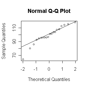
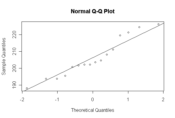
Since the Normal QQ plot with n = 16 observations is as close to a straight line as any of the samples of size 20 plotted above in Question 2, this plot gives us no reason to reject the hypothesis of a Normal distribution.
Using the properties of the exponential distribution, letting T be the time to failure after you buy the car,
(a) P(T < 6) = 1 - exp(-6/6) = 0.632
(b) The mean time to the next failure is 6 years, regardless of the age of the regulator or any other past history.
(a) For a centered 6-sigma process, the probability of not meeting specification, assuming Normality, is, in parts per million
> (pnorm(-6)+pnorm(6,low=F))*1e6
[1] 0.001973175
(b) For the same process, shifted upward by 1.5 standard deviations, the probability is, in parts per million
> (pnorm(-7.5)+pnorm(4.5,low=F))*1e6
[1] 3.397673