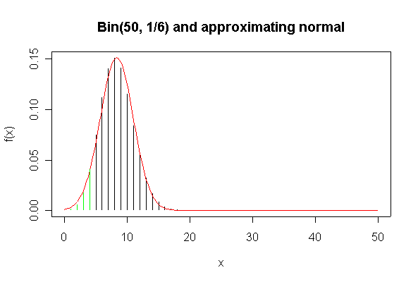
Marks are indicated in red. Full marks = 90.
The normal approximation to the Bin(50, 1/6) distribution is very close graphically; the normal approximation to P(X < 4) = 0.0643 is a bit better with (0.0729) than without (0.0500) the continuity correction.
> plot(0:50,dbinom(0:50,50,1/6),type="h",xlab="x",ylab="f(x)")
> lines(seq(0,50,len=200),dnorm(seq(0,50,len=200),50/6,sqrt(50*5/36)),col="red")
> lines(0:4,dbinom(0:4,50,1/6),type="h",col="green")
> title(main="Bin(50, 1/6) and approximating normal")
> pbinom(4, 50, 1/6)
[1] 0.06431339
> pnorm(4.5, 50/6, sqrt(250/36))
[1] 0.0728834
> pnorm(4, 50/6, sqrt(250/36))
[1] 0.05004841
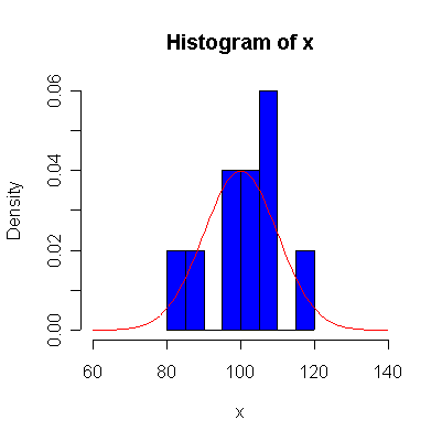
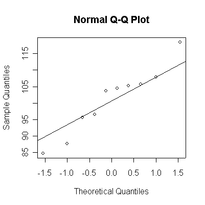
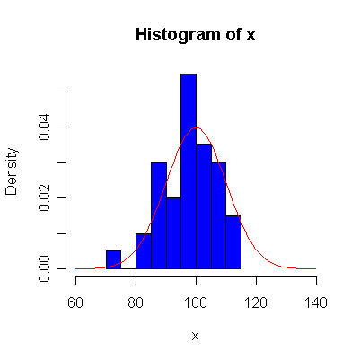
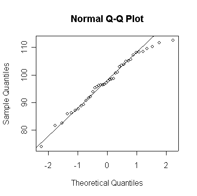
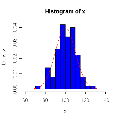
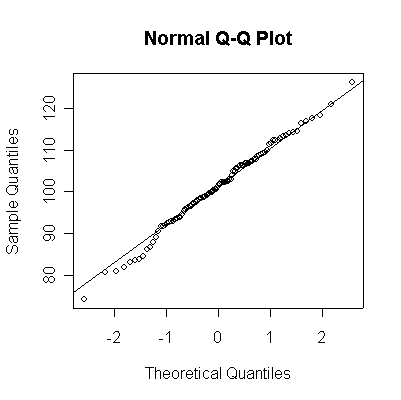
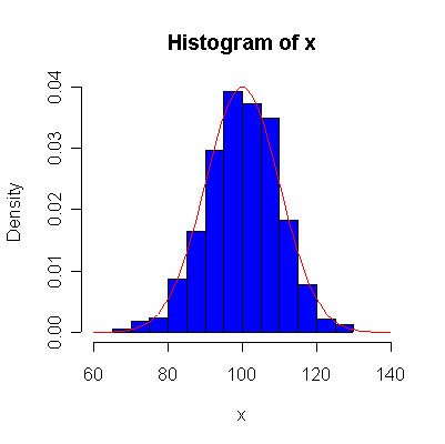
For convenience, I wrote a function normhist() to draw a histogram and superimpose a normal density with given mean and standard deviation, then used this function and qqnorm() and qqline() to give histograms and probability plots for samples of size n = 10, 40, 100, 1000 from the N(100, 10) distribution.
> normhist <-
function (x, mu = 0, sigma = 1)
{
   xgr <- seq(mu - 4 * sigma, mu + 4 * sigma, len = 80)
   hist(x, freq = F, col = "blue", xlim = c(xgr[1], xgr[80]))
   lines(xgr, dnorm(xgr, mu, sigma), col = "red")
   invisible()
}
> xx <- rnorm(10, 100, 10)
> normhist(xx, 100, 10)
> qqnorm(xx)
> qqline(xx)
> xx <- rnorm(40, 100, 10)
> normhist(xx, 100, 10)
> qqnorm(xx)
> qqline(xx)
> xx <- rnorm(100, 100, 10)
> normhist(xx, 100, 10)
> qqnorm(xx)
> qqline(xx)
> xx <- rnorm(1000, 100, 10)
> normhist(xx, 100, 10)
> qqnorm(xx)
> qqline(xx)
 n = 10 n = 10 |
 |
 n = 40 n = 40 |
 |
 n = 100 n = 100 |
 |
 n =
1000 n =
1000 |
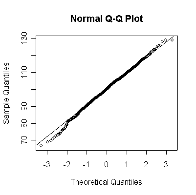 |
Not until n = 100 does the histogram begin to look Normal, and even then it may be skewed one way or the other. The QQ plot is reasonably straight when n = 40, except for the tails of the distribution. This suggests that at least 40 observations, but preferably 100 or more, are needed to demonstrate Normality.
You can do this by hand, but it is tedious. A simple way to list every possible outcome when 3 fair six-sided dice are rolled is to use expand.grid(); here only the first 10 and last 10 rows of the array are shown. All of the 216 possible outcomes are, by symmetry, equally likely.
> expand.grid(1:6,1:6,1:6)
    Var1 Var2 Var3
1      1    1    1
2      2    1    1
3      3    1    1
4      4    1    1
5      5    1    1
6      6    1    1
7      1    2    1
8      2    2    1
9      3    2    1
10     4    2    1
...
207    3    5    6
208    4    5    6
209    5    5    6
210    6    5    6
211    1    6    6
212    2    6    6
213    3    6    6
214    4    6    6
215    5    6    6
216    6    6    6
The following command line generates an array with the 6^3 = 216 possible samples, uses apply() to compute the total score for each sample by summing the rows, then table() to calculate the frequency of each possible score, divides by 6^3 to convert frequency to probability and, finally, calls barplot() to draw the graph.
> barplot(table(apply(expand.grid(1:6,1:6,1:6),1,sum))/(6^3))
The exact mean = 10.5, variance = 8.75 and standard deviation = 2.95804 of this distribution can be computed directly from the probability distribution.
> sum((3:18)*table(apply(expand.grid(1:6,1:6,1:6),1,sum))/(6^3))
[1] 10.5
> sum((((3:18)-10.5)^2)*table(apply(expand.grid(1:6,1:6,1:6),1,sum))/(6^3))
[1] 8.75
> sqrt(sum((((3:18)-10.5)^2)*table(apply(expand.grid(1:6,1:6,1:6),1,sum))/(6^3)))
[1] 2.95804
[An easier way is to calculate mean = 21/6 = 3.5 and variance = 35/12 = 2.916667 for the score on a single die, then multiply by 3 to get mean = 10.5 and variance = 35/4 = 8.75 for the total score on 3 independent dice.]
To simulate 1000 rolls of 3 dice, use sample() to generate 3000 independent rolls of a single die. Arrange them in a matrix with three columns so that summing the rows with apply() gives a vector of total scores for three rolls. Use table() to create a histogram, divide the frequencies by 1000 to make them probabilities, and use barplot() to draw the distribution. Instead of barplot() you could use hist() for this, forcing the break points to be at half-integers, or you could use plot() with type="h". The default histogram isn't always good for discrete distributions. Note that the sample mean = 10.684, sample variance = 8.332 and sample standard deviation = 2.887 are close to their theoretical values.
> dice3 <- apply(matrix(sample(1:6, 1000*3, repl=T), ncol=3), 1, sum)
> barplot(table(dice3)/1000)
> hist(dice3, freq=F)
> plot(table(dice3)/1000, type="h")
> mean(dice3)
[1] 10.684
> var(dice3)
[1] 8.332476
> sqrt(var(dice3))
[1] 2.886603
The Chisq(3) distribution has mean = 3 and variance = 6.
> xgr <- seq(0, 10, length=100)
> plot(xgr, dchisq(xgr,3), type="l", main="Chi-square on 3 degrees of freedom")
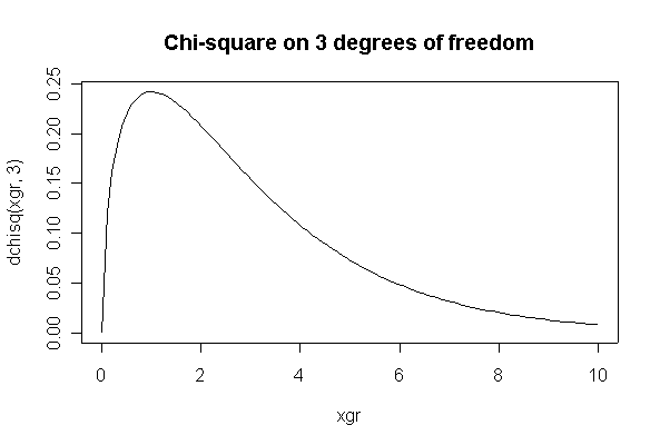
The Central Limit Theorem states that if n = 100, the distribution of the sample mean will be approximately Normal with mean = 3 and standard deviation = sqrt(6/100) = 0.2450.
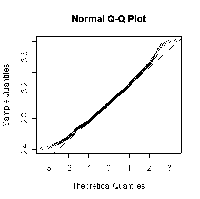
Here we have 1000 realizations of the sample mean; the histogram and Normal QQ plot indicate that the sampling distribution is very close to Normal, even though the data came from a non-normal distribution. The observed mean of 3.001 and standard deviation of 0.2391 are close to their theoretical values of 3 and 0.2450, respectively.
> chisq3means <- apply(matrix(rchisq(1000*100, 3), ncol=100), 1, mean)
> normhist(chisq3means, 3, sqrt(6/100))
> qqnorm(chisq3means)
> qqline(chisq3means)
> mean(chisq3means)
[1] 3.001238
> sqrt(var(chisq3means))
[1] 0.2390889
 |
 |
Define the events A: process A operating, B: process B operating, C: process C operating, D: process D operating; P: dangerous pollution products produced; K: fish kill. We are given that events A, B, C, D are mutually exclusive and P(A) = 0.2, P(B) = 0.4, P(C) = 0.3, P(D) = 0.1. Also, P(P|A) = 0.4, P(P|B) = 0.05, P(P|C) = 0.3, P(P|D) = 0.1. Let ' denote complementary event, so P' means "no dangerous pollution products produced." Let AP denote the intersection of A and P, "process A operating and producing dangerous pollution products," etc.
We are also given that P(K|AP) = 0.9, P(K|BP) = 0.1, P(A|CP) = 0.8, P(K|DP) = 0.3.
(a) P(no dangerous pollution discharge in a given month) = P(P') = 1 - P(P) = 1 - [P(P|A)P(A) + P(P|B)P(B) + P(P|C)P(C) + P(P|D)P(D)] = 1 - 0.2 = 0.8
(b) P(A) = 0.2 but P(A|P) = P(P|A)P(A)/P(P) = 0.4*0.2/0.2 = 0.4
(c) P(K) = P(KAP) + P(KBP) + P(KCP) + P(KDP)
= P(K|AP)P(P|A)P(A) + P(K|BP)P(P|B)P(B) + P(K|CP)P(P|C)P(C) +
P(K|DP)P(P|D)P(D)
= 0.072 + 0.002 + 0.072 + 0.003 = 0.149
Thus the probability of a fish kill in a given month is 14.9%. Processes A and C make the largest contribution to this sum, the probability of a Process A fish kill in a given month being 7.2% while the probability of a Process C fish kill is also 7.2%, so either could be considered for cleanup. Of the two, Process A has the higher probability of dangerous pollution and the higher probability of a fish kill if it does pollute so it may be most fruitful to begin by cleaning up Process A.
Assuming that accidents occur independently, one at a time, at a constant average rate, the accidents form a Poisson Process with rate = 1/6 per month. I have used R here; be sure that you know how to do these calculations on a calculator, they are very simple.
(a) Let X = number of accidents in 4 months; X ~ Pois(4/6), so P(X = 1) = 0.342 or 34.2%.
(b) P(X >= 1) = 1 - P(X = 0) = 0.487 or 48.7%.
(c) Let Y = number of accidents in 12 months; Y ~ Pois(12/6), so the mean is 2 per year and the standard deviation is sqrt(2) = 1.414.
(d) P(wins award next year) = P(Y = 0) = 0.135 or 13.5%.
(e) Let W = number of time he wins the award in the next 5 years; W ~ Bin(5, P(Y = 0)) so P(W = 2) = 0.118 or 11.8%.
> dpois(1, 4*(1/6))
[1] 0.3422781
> 1-ppois(0, 4*(1/6))
[1] 0.4865829
> dpois(0, 12*(1/6))
[1] 0.1353353
> dbinom(2, 5, dpois(0, 12*(1/6)))
[1] 0.1184037
Let X be the number of ticket holders who show up for the flight; from the assumptions given, X ~ Bin(125, 0.9).
(a) P(every passenger who shows up gets a seat) = P(X <= 120) = 0.996
> pbinom(120, 125, 0.9)
[1] 0.9961414
(b) P(empty seats) = P(X < 120) = P(X <= 119) = 0.989
> pbinom(119, 125, 0.9)
[1] 0.9885678
Let X be compressive strength in Kg/cm2; we are given that X ~ N(6000, 100^2). Here are answers using Table II on p. 653 and using R.
(a) P(X < 6250) = Φ((6250-6000)/100) = Φ(2.5) = 0.993790
> pnorm(6250, 6000, 100)
[1] 0.9937903
(b) P(5800 < X < 5900) = Φ((5900-6000)/100) - Φ((5800-6000)/100)= Φ(-1) - Φ(-2) = 0.158655 - 0.022750 = 0.135905
> pnorm(5900, 6000, 100) - pnorm(5800, 6000, 100)
[1] 0.1359051
(c) From the bottom line of Table IV on p. 656, the 5th percentile of the standard normal is -1.645, so the strength exceeded by 95% of the samples is
-1.645*100 + 6000 = 5835.5 Kg/cm2
> qnorm(.05, 6000, 100)
[1] 5835.515
Let X be the number of exposed people who become ill. From the assumptions given, X ~ Bin(1000, 0.2) which is approximately N(200, 160). Here are the exact calculations and their normal approximations (with continuity correction).
(a) P(X > 225)
> 1-pbinom(225,1000,.2)
[1] 0.02311485
> 1-pnorm(225.5,200,sqrt(160))
[1] 0.02190250
(b) P(175 < X < 225)
> pbinom(225,1000,.2) - pbinom(174,1000,.2)
[1] 0.9563079
> pnorm(225.5,200,sqrt(160)) - pnorm(174.5,200,sqrt(160))
[1] 0.956195
(c) The 99th percentile is not defined exactly for a discrete distribution. It can be found by trial and error, or as a binomial quantile using R, or approoximately as a normal quantile using R, or approximately from the normal tables. (The 99th percentile of the standard normal is 2.326, from the bottom line of Table IV on p.656.) The calculations below show that the chance that more than 230 people become ill is slightly less than 0.01, the chance that more than 229 people become ill is slightly greater than 0.01, so either 229 or 230 is an acceptable answer. Only the last calculation, using the standard normal quantile from Table IV, is suitable for hand calculation.
> qbinom(.99,1000,.2)
[1] 230
> pbinom(230,1000,.2)
[1] 0.9912482
> pbinom(229,1000,.2)
[1] 0.9892641
> qnorm(.99,200,sqrt(160)) - .5
[1] 228.9262
> qnorm(.99)
[1] 2.326348
> 200+2.326*sqrt(160) - .5
[1] 228.9218
(a) For a centered 6-sigma process, the probability of not meeting specification, assuming Normality, is, in parts per million
> (pnorm(-6)+pnorm(6,low=F))*1e6
[1] 0.001973175
(b) For the same process shifted upward by 1.5 standard deviations, the probability is, in parts per million
> (pnorm(-6-1.5)+pnorm(6-1.5,low=F))*1e6
[1] 3.397673
(c) For a centered 3-sigma process, the probability of not meeting specification, assuming Normality, is, in parts per million
> (pnorm(-3)+pnorm(3,low=F))*1e6
[1] 2699.796
(d) For the same process shifted upward by 1.5 standard deviations, the probability is, in parts per million
> (pnorm(-3-1.5)+pnorm(3-1.5,low=F))*1e6
[1] 66810.6
(e) It is almost impossible for a process running at six-sigma quality to depart from specification if it is centred. Even if the mean shifts by 1.5 standard deviations the chance is only 3 parts per million. If the process were running at three-sigma quality, these probabilities would be many orders of magnitude larger.