> xgr <- seq(-4,4,length=50)
> plot(xgr, dnorm(xgr), type = "l", lty = 1, xlab = "x", ylab ="f(x)")
> lines(xgr,dt(xgr,10),lty=2)
> lines(xgr,dt(xgr,1),lty=3)
> legend(1.8,.38,c("infinite df","10 df","1 df"),lty=1:3)
> title("t density")
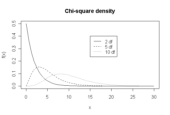
> xgr <- seq(0,30,length=50)
> plot(xgr, dchisq(xgr, 2), type = "l", lty = 1, xlab = "x", ylab ="f(x)")
> lines(xgr,dchisq(xgr,5),lty=2)
> lines(xgr,dchisq(xgr,10),lty=3)
> legend(15,.4,c("2 df","5 df","10 df"),lty=1:3)
> title("Chi-square density")
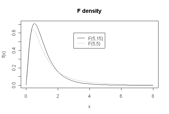
> xgr <- seq(0,8,length=90)
> plot(xgr, df(xgr,5,15), type = "l", lty = 1, xlab = "x", ylab ="f(x)")
> lines(xgr,df(xgr,5,5),lty=3)
> legend(3,.6,c("F(5,15)","F(5,5)"),lty=c(1,3))
> title("F density")
The confidence interval is (29.48, 47.92).
> qt(.975,8)*12/sqrt(9)
[1] 9.224016
> 38.7 + c(-1,1)*qt(.975,8)*12/sqrt(9)
[1] 29.47598 47.92402
To solve for the sample size, we have to solve qt(.975, n-1)*12/sqrt(n)
= 2 to get n. This is complicated because we have to know n
to get qt(.975, n-1), but we know that if n is large
qt(.975, n-1) will be close to 2 and this gives the solution n =
144. (If the solution were not an integer, we would round up to the next
integer.)
> (2*12/2)^2
[1] 144
When the process mean is 100 g, the probability that a given pellet is within limits is 0.8904, and this becomes 0.7799 when the mean shifts to 102 g. Compute the binomial probability of getting exactly 1 out of 4 pellets within the limits for the normal process and for the shifted process, then use Bayes' Theorem to compute the probability that the process mean has shifted, given that 1 out of 4 was within the limits. The answer is 44.06%.
> pr1 <- pnorm(104,100,2.5)-pnorm(96,100,2.5)
> pr1
[1] 0.8904014
> pr2 <- pnorm(104,102,2.5)-pnorm(96,102,2.5)
> pr2
[1] 0.779947
> dbinom(1,4,pr1)
[1] 0.004688789
> dbinom(1,4,pr2)
[1] 0.03324349
> dbinom(1,4,pr2)*0.1/(dbinom(1,4,pr2)*0.1 + dbinom(1,4,pr1)*0.9)
[1] 0.4406462
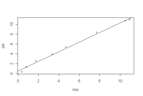
Either a paired t-test or a simple linear regression is a valid analysis; a two-sample t-test is NOT valid.
> chlorine
    msi   sib  diff
1  0.39  0.36 -0.03
2  0.84  1.35  0.51
3  1.76  2.56  0.80
4  3.35  3.92  0.57
5  4.69  5.35  0.66
6  7.70  8.33  0.63
7 10.52 10.70  0.18
8 10.92 10.91 -0.01
> t.test(chlorine$sib,chlorine$msi,pair=T)

        Paired t-test

data:  chlorine$sib and chlorine$msi
t = 3.6454, df = 7, p-value = 0.008228
alternative hypothesis: true difference in means is not equal to 0
95 percent confidence interval:
 0.1453686 0.6821314
sample estimates:
mean of the differences
                0.41375

> stem(chlorine$diff)

  The decimal point is 1 digit(s) to the left of the |

  -0 | 31
   0 | 8
   2 |
   4 | 17
   6 | 36
   8 | 0
Assumptions:
Conclusions:
There is evidence (P = 0.008) that mean MSI and mean SIB are not equal.
> fitchlor<-lm(sib~msi,chlorine)
> summary(fitchlor)

Call:
lm(formula = sib ~ msi, data = chlorine)

Residuals:
     Min       1Q   Median       3Q      Max
-0.56096 -0.13956  0.05219  0.24941  0.30371

Coefficients:
            Estimate Std. Error t value Pr(>|t|)
(Intercept)  0.54083    0.18705   2.891   0.0276 *
msi          0.97469    0.02928  33.283  4.9e-08 ***
---
Signif. codes:  0 `***' 0.001 `**' 0.01 `*' 0.05 `.' 0.1 ` ' 1

Residual standard error: 0.327 on 6 degrees of freedom
Multiple R-Squared: 0.9946,     Adjusted R-squared: 0.9937
F-statistic:  1108 on 1 and 6 DF,  p-value: 4.895e-08

> plot(sib~msi, data=chlorine)
> abline(fitchlor)
Assumptions:
Conclusions:
There is strong evidence of a linear relationship between MSI and SIB, the slope is very close to 1 but the intercept is not zero.
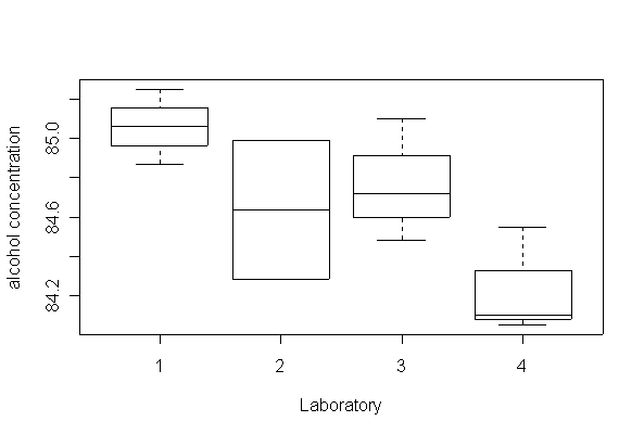
The correct analysis is as a single factor ANOVA; the missing value can be omitted, leaving the design unbalanced.
> alcohol
    conc lab
1  85.06   1
2  85.25   1
3  84.87   1
4  84.99   2
5  84.28   2
6  84.48   3
7  84.72   3
8  85.10   3
9  84.10   4
10 84.55   4
11 84.05   4

> anova(lm(conc~as.factor(lab), data=alcohol))
Analysis of Variance Table

Response: conc
          Df  Sum Sq Mean Sq F value Pr(>F)
lab        3 1.05823 0.35274  3.6778 0.0708 .
Residuals  7 0.67138 0.09591
---
Signif. codes:  0 `***' 0.001 `**' 0.01 `*' 0.05 `.' 0.1 ` ' 1

> boxplot(conc~lab, data=alcohol, ylab="alcohol concentration", xlab="Laboratory")
Assumptions:
Conclusions:
There is some evidence (P = 0.07) that the 4 labs do not all give the same mean % alcohol determination.
Note how the residual mean square can be extracted as entry [3,3] of the ANOVA table, and upper and lower 95% confidence limits (0.0571, 0.6673) computed in a single statement. The "as.factor(age)" line in the ANOVA table is the lack of fit test, it comes from adding age as a factor to the model after age as linear regressor.
> pipecrack
  age  load
1  20 11.45
2  20 10.42
3  20 11.14
4  25 10.84
5  25 11.17
6  25 10.54
7  31  9.47
8  31  9.19
9  31  9.54

> plot(load~age, data=pipecrack)
> anova(lm(load~age+as.factor(age), data=pipecrack))
Analysis of Variance Table

Response: load
               Df Sum Sq Mean Sq F value   Pr(>F)
age             1 4.0362  4.0362 29.3306 0.001639 **
as.factor(age)  1 0.6605  0.6605  4.7996 0.070997 .
Residuals       6 0.8257  0.1376
---
Signif. codes:  0 `***' 0.001 `**' 0.01 `*' 0.05 `.' 0.1 ` ' 1
> mseq3<-anova(lm(load~age+as.factor(age),pipecrack))[3,3]
> mseq3

0.1376111
> 6*mseq3/c(qchisq(.975,6),qchisq(.025,6))
[1] 0.05714203 0.66728937
> abline(lm(load~age, data=pipecrack))
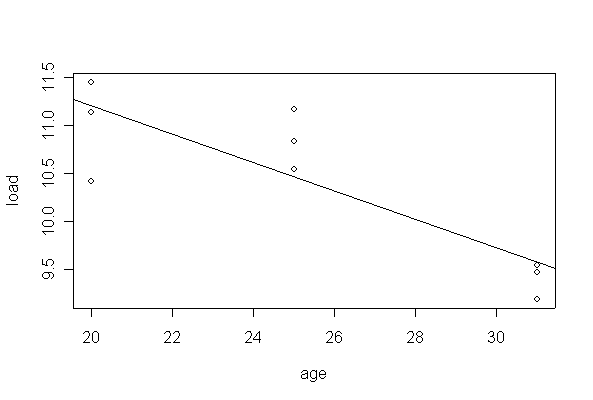
Since the lack of fit test did not reject the hypothesis of linearity, an alternative analysis without the lack of fit sum of squares is valid; this gives 7 df for the residual mean square, and a different confidence interval for the residual variance (0.0928, 0.8794) based on 7 df.
> anova(lm(load~age, data=pipecrack))
Analysis of Variance Table

Response: load
          Df Sum Sq Mean Sq F value   Pr(>F)
age        1 4.0362  4.0362  19.011 0.003313 **
Residuals  7 1.4861  0.2123
---
Signif. codes:  0 `***' 0.001 `**' 0.01 `*' 0.05 `.' 0.1 ` ' 1

> 7*anova(lm(load~age,pipecrack))[2,3]/c(qchisq(.975,7),qchisq(.025,7))
[1] 0.0928099 0.8794427
>
> coef(lm(load~age,pipecrack))
(Intercept)         age
 14.1904029  -0.1489194
> summary(lm(load~age,pipecrack))

Call:
lm(formula = load ~ age, data = pipecrack)

Residuals:
    Min      1Q  Median      3Q     Max
-0.7920 -0.1039 -0.0339  0.2380  0.7026

Coefficients:
            Estimate Std. Error t value Pr(>|t|)
(Intercept) 14.19040    0.87877   16.15  8.5e-07 ***
age         -0.14892    0.03415   -4.36  0.00331 **
---
Signif. codes:  0 `***' 0.001 `**' 0.01 `*' 0.05 `.' 0.1 ` ' 1

Residual standard error: 0.4608 on 7 degrees of freedom
Multiple R-Squared: 0.7309,     Adjusted R-squared: 0.6924
F-statistic: 19.01 on 1 and 7 DF,  p-value: 0.003313
Some evidence of nonlinearity (P = 0.07) but the hypothesis of linearity over the range of ages studied is acceptable at the 5% level. There is evidence (P < 0.01) that load at first crack decreases with age of pipe.
Note how in R the new age values to be used for the prediction have to be supplied in a data frame.
> predict(lm(load~age, pipecrack), newdata=data.frame(age=c(22,100)))
         1          2
10.9141758 -0.7015385
The prediction at 22 days is an interpolation so it might be OK, except that the true relationship may not be exactly linear. The prediction at 100 days is an extreme extrapolation which gives an impossible negative value, so it is not reliable and should not be used.
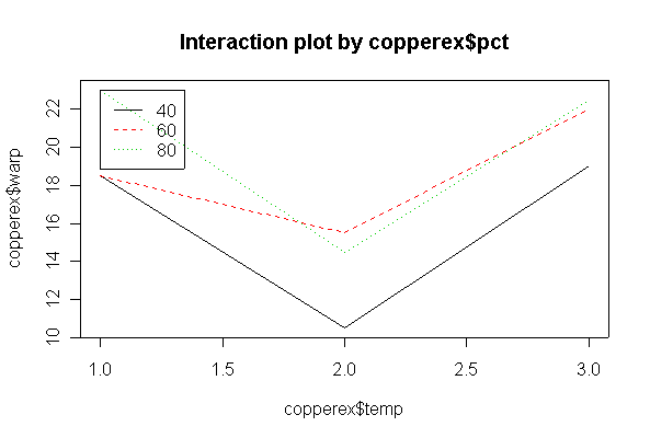
The analysis is as a two-factor design with interaction. The 95% CI for the residual variance is (3.101, 21.85) on 9 df.
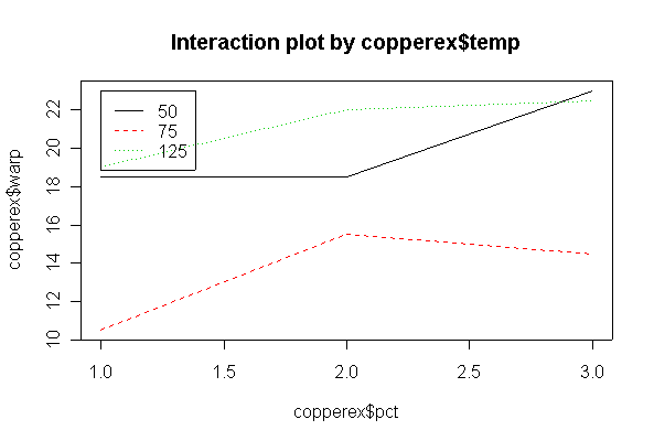
> copperex
   warp temp pct
1    17   50  40
2    20   50  40
3    16   50  60
4    21   50  60
5    24   50  80
6    22   50  80
9    12   75  40
10    9   75  40
11   18   75  60
12   13   75  60
13   17   75  80
14   12   75  80
25   21  125  40
26   17  125  40
27   23  125  60
28   21  125  60
29   23  125  80
30   22  125  80
> copperex$temp <- as.factor(copperex$temp)
> copperex$pct <- as.factor(copperex$pct)
> interactplot(copperex$warp, copperex$pct, copperex$temp)
> interactplot(copperex$warp, copperex$temp, copperex$pct)
> anova(lm(warp~pct*temp, data=copperex))
Analysis of Variance Table

Response: warp
          Df  Sum Sq Mean Sq F value   Pr(>F)
pct        2  49.778  24.889  3.7966 0.063739 .
temp       2 204.778 102.389 15.6186 0.001184 **
pct:temp   4  19.556   4.889  0.7458 0.584683
Residuals  9  59.000   6.556
---
Signif. codes:  0 `***' 0.001 `**' 0.01 `*' 0.05 `.' 0.1 ` ' 1
> anova(lm(warp~pct*temp,copperex))[4,3]

6.555556
> 9*anova(lm(warp~pct*temp,copperex))[4,3]/c(qchisq(.975,9),qchisq(.025,9))
[1]  3.101547 21.848700
There is no evidence (P = 0.585) from these data that % copper and temperature interact. There is strong evidence (P = 0.001) that temperature affects warping, but less evidence (P = 0.064) that % copper affects warping, over the range of % copper studied.
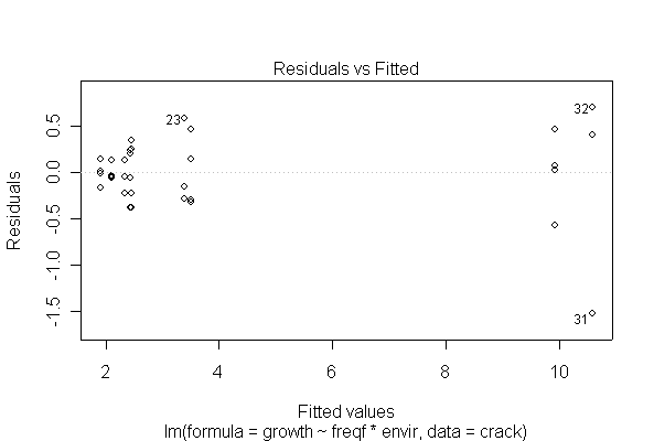
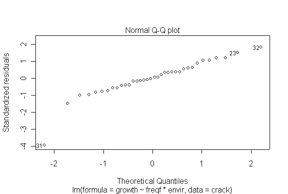
The analysis is as a two-factor design with interaction. The interaction is significant at the 5% level, and is in fact highly significant, so there is no need to test the main effects separately. Cyclic loading frequency and environmental conditions both affect fatigue crack growth, and the effect of loading frequency is different under different environments. The ANOVA tables from untransformed and log-transformed data are almost the same.
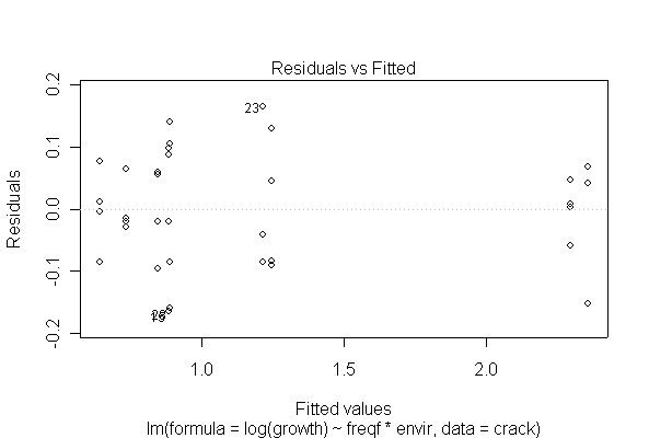
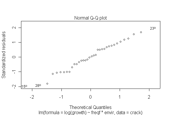
I have shown two of the diagnostic plots, "Residuals vs. Fitted" and a Normal probability plot of the residuals. You are not expected to do the residual plots by hand. The log-transformed data are more homoscedastic and more normal than the untransformed data, and one outlier (observation #31) is pulled in closer to the rest of the data, but that does not seem to affect the analysis very much.
(In Assignment #1 you did a simple graphical analysis of these data; does this more sophisticated analysis tell us anything more than the graphical analysis?)
> fitcrack <- lm(growth~freqf*envir, data=crack)
> anova(fitcrack)
Analysis of Variance Table

Response: growth
            Df  Sum Sq Mean Sq F value    Pr(>F)
freqf        2 209.893 104.946  522.40 < 2.2e-16 ***
envir        2  64.252  32.126  159.92 1.076e-15 ***
freqf:envir  4 101.966  25.491  126.89 < 2.2e-16 ***
Residuals   27   5.424   0.201
---
Signif. codes:  0 `***' 0.001 `**' 0.01 `*' 0.05 `.' 0.1 ` ' 1
> plot(fitcrack)
> fitcrackl <- lm(log(growth)~freqf*envir, data=crack)
> anova(fitcrackl)
Analysis of Variance Table

Response: log(growth)
            Df Sum Sq Mean Sq F value    Pr(>F)
freqf        2 7.5702  3.7851 404.095 < 2.2e-16 ***
envir        2 2.3576  1.1788 125.849 2.061e-14 ***
freqf:envir  4 3.5284  0.8821  94.172 1.885e-15 ***
Residuals   27 0.2529  0.0094
---
Signif. codes:  0 `***' 0.001 `**' 0.01 `*' 0.05 `.' 0.1 ` ' 1
> plot(fitcrackl)