Univariate (one-dimensional), discrete-time, deterministic model: N(t + 1) = f(N(t)). (Typically, state variable is continuous.) (Units of time, stock? When does discrete time make sense?)

Geometric growth (decay)

Simplest possible model. f(N) = RN (sometimes stated as f(N) = (1 + r)N). Solve recursion analytically. Now we know everything about the dynamics. Suppose N(0) > 0, R > 0 (note: the R language indexes vectors starting from 1). (What happens if N(0) < 0 ? model of debt?)

What happens if R < 0?

(Even this ridiculously simple rule — or generalizations of it — is the basis of serious modeling in conservation biology.)

The limiting set of points as t →∞ is called an attractor. If R < 1, N → 0 but N = 0 only in the limit, unless it starts there. A value of N such that f(N^*) = N^* is called an equilibrium (or a fixed point).

Stability: what happens for perturbations in the neighborhood of the fixed point? Consider displacing the population away from N^* by δ, where δ ≪ 1; what happens?

Therefore the deviation δ → δf′(N^*). If |g|≡|f′(N^*)| < 1 then the deviation from the equilibrium decreases geometrically with time: stable fixed point. Behavior for g < (-1), -1 < g < 0, 0 < g < 1, g > 1 …

N = 0 is always an equilibrium, stable iff |R| < 1.

Affine models

Now suppose (as in the example in the book) we are adding or subtracting a fixed amount per time step: N(t + 1) = a + bN(t). As before we can work out the recursion.

Summing the series for t steps gives a(1 -b^t)∕(1 -b) + b^tN; the limit is a∕(1 -b) + lim_t→∞b^tN(0). If |b| > 1 this is a bit boring. If |b| < 1 we get a stable equilibrium at a∕(1 -b). (For b < 0 (“bucket model”): a is the supply rate, 1∕(1 - b) is the average residence time.)

Useful component for larger models. (Autoregressive model in time series analysis; sometimes used as the bottom level in food chain modeling.)

In general, things are not so simple. The general approach is (1) solve for equilibria (directly); (2) evaluate stability of equilibria; (3) possibly evaluate for small N (near system boundaries); (4) if possible solve for time-dependent solution.

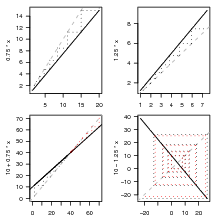
Graphical approaches: cobwebbing

Multiple lags

What if N(t + 1) depends on previous time steps N(t - 1) etc. as well as N(t)? Homogeneous linear equations: ∑ _i=0^ma_iN(t - i) = 0. Plug in N(t) = Cλ^t. Solve characteristic equation …get a linear combination of geometric growth/decay, ∑ C_iλ_iⁿ: largest eigenvalue dominates long-term behavior.