Logistic model
Impose bounds on an otherwise ridiculous growth process. (Mechanistic/phenomenological description.) N(t) = N + rN(1 -N∕K); can set K = 1 (non-dimensionalization). Get expected results for R < 1, R small (< 2). (Equilibrium?)
Alternative parameterizations
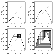
An ecologist or other normal person might choose to parameterize the discrete logistic model as above. A mathematician would choose x(t + 1) = Rx(1 - x). The mathematician has chosen R = r∕K → K = 1 - 1∕R. Mathematically equivalent parameterizations often have quite different meanings (or statistical properties), as well as cultural connotations. Get used to it.
More nonlinear models
Other 1-D discrete nonlinear models: Ricker model (N = rNe-bN); population genetics; approximations of continuous models. Epidemic models (SI) (equivalent to discrete logistic).
Graphical approaches, continued: Allee effects. Bistability, multiple stable states.
Linear multi-state/multi-lag models
Back to linear models (briefly). Juvenile/adult model: fractions {sJ,sA} of juveniles and adults survive; adults have
f offspring each (on average); surviving juveniles become adults. So A(t + 1) = sAA(t) + sJJ(t), J(t + 1) = fA(t) or
A(t + 1) = sAA(t) + sJfA(t- 1). Could try to solve by recursion. Or guess that the solutions are of the form Cλt.
Plug in: Cλt+1 = sACλt + sJfCλt-1, or λ2 -sAλ-sJf = 0 (characteristic equation). λ = 1∕2(sA ± ).
CE is the same as if we wrote it in the multi-state, matrix form: N = MN where M =
).
CE is the same as if we wrote it in the multi-state, matrix form: N = MN where M =  ; then the
solutions of the CE are the eigenvalues of M (i.e. values of λ s.t. Mv = λv for some eigenvector v). Solution is a
mixture: A(t) = C+λ+t + C-λ-t.
; then the
solutions of the CE are the eigenvalues of M (i.e. values of λ s.t. Mv = λv for some eigenvector v). Solution is a
mixture: A(t) = C+λ+t + C-λ-t.
What can we say about λ±? Can put in values (e.g. sA = 0.9, sJ = 0.5, f = 2; then the eigenvalues are (0.9 ± 2.19)∕2 = {1.55,-0.65}.
Nonlinear multi-state models
Things get interesting now: e.g. epidemic model, S(t + 1) = S + (mN -mS -βSI), I(t + 1) = I + (βSI -mI -γI).
Equilibria: straightforward algebra (solve f(S*,I*) = {S*,I*}). Stability: linearization of f(S,I) near {S*,I*}.