Definitions

1. In general for two events A and B the probability of both occurring is Prob(A ∪ B) = Prob(A) + Prob(B) - Prob(A ∩ B), where the last bit term is the joint probability of A and B.
2. For mutually exclusive events (joint prob. = 0, e.g., “individual is male/female”); probability of A or B ≡ Prob(A ∪ B) = Prob(A) + Prob(B).
3. The sum of probabilities of all possible outcomes of an observation or experiment = 1.0. (E.g.: normalization constants.)
4. Conditional probability of A given B, Prob(A|B): Prob(A|B) = Prob(A∩B)∕Prob(B). (Compare the unconditional probability of A: Prob(A) = Prob(A|B) + Prob(A|not B).)
5. If Prob(A|B) = Prob(A), A is independent of B. Independence ⇐⇒ Prob(A ∩ B) = Prob(A)Prob(B) (or log ∏ _iProb(A_i) = ∑ _i log Prob(A_i)).

Probability distributions

Discrete: probability distribution, cumulative probability distribution. Continuous: cumulative distribution function, probability density function (p(x) = limit of Prob(x < X < x + Δx)∕Δx as Δx → 0).

Moments: Means: ∑ x_i∕N = ∑ count(x)x∕N = ∑ p(x)x (discrete), ∫ p(x)xdx. Variances: ∑ p(x)(x -x)², ∫ p(x)(x -x)²dx. Higher moments: skew, kurtosis.

Other descriptors: median, mode.

Bestiary

Pretty good summaries on Wikipedia (http://en.wikipedia.org/wiki/List_of_probability_distributions). R help pages. Books: [1, 2], Johnson, Kotz, Balakrishnan et al.

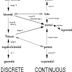
Characteristics (discrete vs continuous; range (positive, bounded, …); symmetric or skewed …)

• Binomial: independent trials from fixed number of trials N with homogeneous per-trial probabilities p (Bernoulli: N = 1).
• Poisson: sample with independent occurrence, homogeneous probability per unit effort (lim N →∞ with Np constant of Binomial).
• Negative binomial: independent homogeneous Bernoulli trials until m successes; overdispersed version of Poisson (Gamma-Poisson).
• Normal (Gaussian): continuous, symmetric; central limit theorem.
• Gamma: waiting time (exponential: shape=1).
• Lognormal: exponential-transformed Gaussian.

(Insanely thorough version: [3].)

Jensen’s inequality

Bottom line: E[f(x)]≠f(E[x]), unless f is linear (need new notation for expectation over a particularly probability density function p(x): E_p[f(x)] ≡∫ p(x)f(x)dx. Quantify exactly by calculating the expectation precisely, or by the delta method.

Delta method: E_p[f(x)] ≈ E_p[f(x)] + E_p[f′(x)|_x=x(x-x)] + 1∕2E_p[f′′(x)|_x=x(x-x)²] = f(x) + 1∕2f′′(x)Var(x).

References

[1] B. M. Bolker. Ecological Models and Data in R. Princeton University Press, 2008.
[2] M. Evans, N. Hastings, C. Forbes, and J. B. Peacock. Statistical Distributions. John Wiley & Sons, 2010.
[3] L. M. Leemis and J. T. McQueston. Univariate distribution relationships. The American Statistician, 62(1):45–53, 2008.