dual_keen

Base Parameters - Table 3
Functions of interest
Other definitions
Example 1
Example 2
Example 3
Auxiliary functions

function out = dual_keen()

%%%%%%%%%%%%%%%%%%%%%%%%%%%%%%%%%%%%%%%%%%%%%%%%%%%%%%%%%%%%%%%%%%%%%%%%%%%
% This code simulates the dual Keen model as specified in
% Giraud and Grasselli (2019)
%
%
% authors: G. Giraud and M. Grasselli
%%%%%%%%%%%%%%%%%%%%%%%%%%%%%%%%%%%%%%%%%%%%%%%%%%%%%%%%%%%%%%%%%%%%%%%%%%%
clear all
close all
clc
warning off

Base Parameters - Table 3

nu = 3;          %capital to output ratio
alpha = 0.025;   %productivity growth rate
beta = 0.02;     %population growth rate
delta = 0.05;    %depreciation rate
r = 0.03;        %real interest rate
eta_p = 0.35;    % adjustment speed for prices
markup = 1.6;    % mark-up value
gamma = 0.8;     % (1-gamma) is the degree of money ilusion

phi0 = 0.04/(1-0.04^2); %Phillips curve parameter
phi1 = 0.04^3/(1-0.04^2); %Phillips curve parameter
c_minus= 0.03; % consumption share hard-lower bound
A_c = 0; %Consumption share asymptotic lower bound
B_c = 5; % Consumption share growth rate
C_c = 1;
K_c = 0.9; %Consumption share upper bound
nu_c = 0.2;
Q_c= ((K_c-A_c)/(c_minus-A_c))^nu_c-C_c;

Functions of interest

fun_consumption =@(x) max(c_minus,A_c + ((K_c-A_c)./(C_c+Q_c*exp(-B_c*x)).^(1/nu_c))); %----first specification : generalised logistic consumption function------%
fun_consumption_inv = @(x) -log((((K_c-A_c)./(x-A_c)).^nu_c-C_c)./Q_c)./B_c; % inverse of the consumption function over positive income

fun_Phi = @(x) phi1./(1-x).^2- phi0;
fun_Phi_prime = @(x) 2*phi1./(1-x).^3;
fun_Phi_inv = @(x) 1 - (phi1./(x+phi0)).^(1/2);

Other definitions

TOL = 1E-7;
options = odeset('RelTol', TOL);
txt_format = '%3.3g';

Example 1

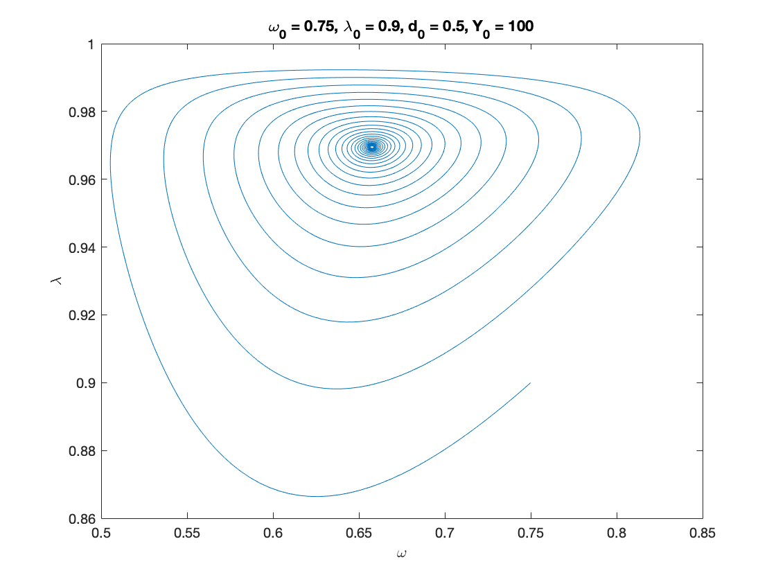
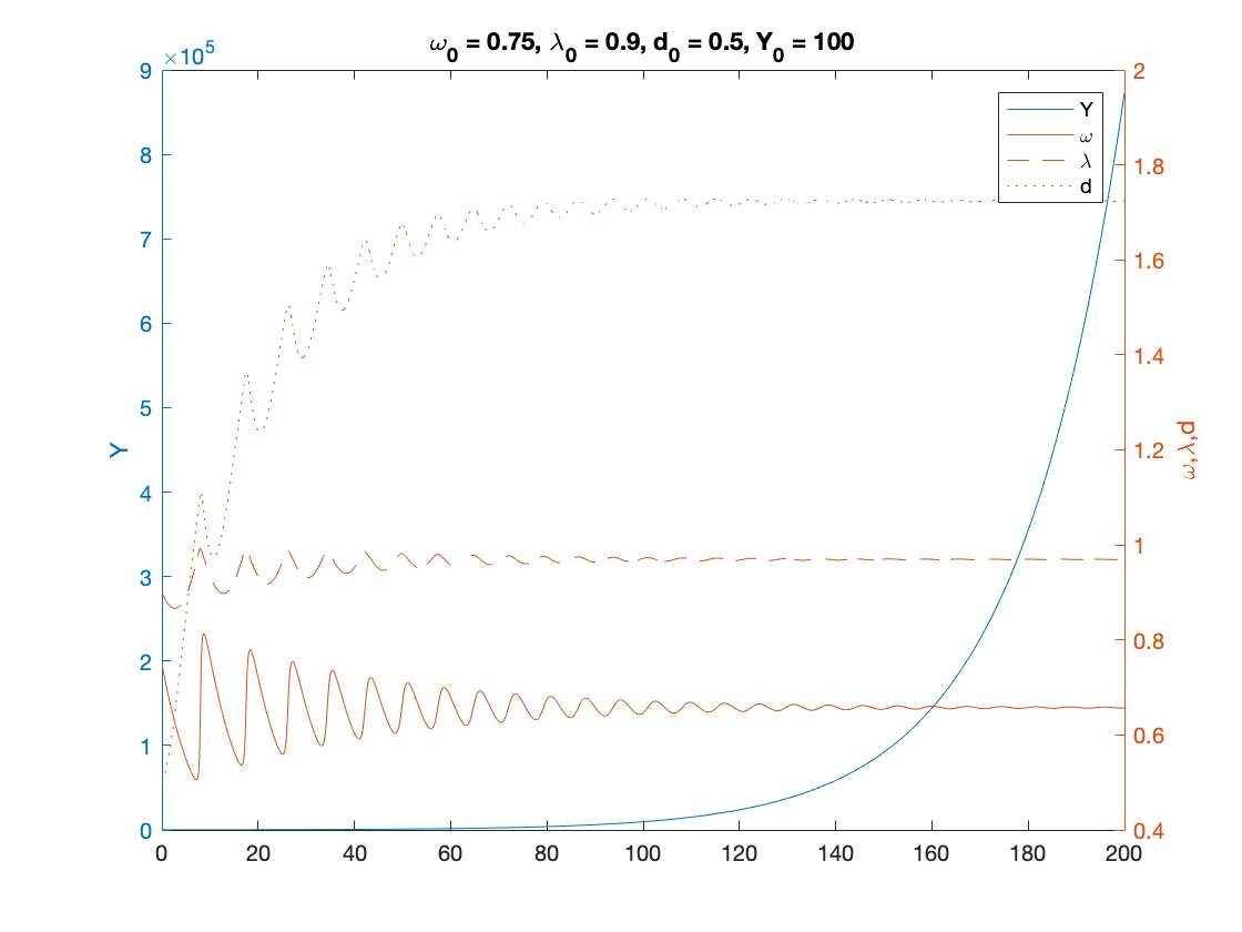
% Parameters as in Table 3
nu = 3;          %capital to output ratio
alpha = 0.025;   %productivity growth rate
beta = 0.02;     %population growth rate
delta = 0.05;    %depreciation rate
r = 0.03;        %real interest rate
eta_p = 0.35;    % adjustment speed for prices
markup = 1.6;    % mark-up value
gamma = 0.8;     % (1-gamma) is the degree of money ilusion

% Numerical Values of Interest
c_eq=1-nu*(alpha+beta+delta)
eta_1 = fun_consumption_inv(c_eq)

A_w = eta_p*markup; % Coefficients in the quadratic equation A_w omega^2 + B_w omega + C_w = 0
B_w = alpha+beta-eta_p*(1+eta_1*markup);
C_w = eta_1*(eta_p-alpha-beta)+r*(eta_1-c_eq);

x=[];
syms x
omega_1 = vpasolve(A_w*x^2+B_w*x+C_w ==0,x)
i_omega_1 = eta_p*(markup*omega_1-1)
g_nominal_1 = alpha+beta+i_omega_1
lambda_1 = fun_Phi_inv(alpha+(1-gamma)*eta_p*(markup*omega_1-1))
d_1 = (omega_1-eta_1)./r

eta_1_calc=omega_1-r.*d_1; % verification step
c_eq_calc=fun_consumption(eta_1_calc); %verification step

% Sample paths of the dual Keen model

omega0 = 0.75;
lambda0 = 0.9;
d0 = 0.5;
Y0 = 100;
T = 200;

[tK,yK] = ode15s(@(t,y) dual_keen(y), [0 T], convert([omega0, lambda0, d0]), options);
yK = retrieve(yK);
Y_output = Y0*yK(:,2)/lambda0.*exp((alpha+beta)*tK);

n=length(yK(:,3))

omega_bar = yK(n,1)
lambda_bar = yK(n,2)
d_bar = yK(n,3)

figure(1)
plot(yK(:,1), yK(:,2)), hold on;
%plot(bar_omega_K, bar_lambda_K, 'ro')
xlabel('\omega')
ylabel('\lambda')
title(['\omega_0 = ', num2str(omega0, txt_format), ...
    ', \lambda_0 = ', num2str(lambda0, txt_format), ...
    ', d_0 = ', num2str(d0, txt_format), ...
    ', Y_0 = ', num2str(Y0, txt_format)])

print('dual_keen_phase_convergent','-depsc')

figure(2)
yyaxis right
plot(tK, yK(:,1),tK,yK(:,2),tK,yK(:,3))
ylabel('\omega,\lambda,d')

yyaxis left
plot(tK, Y_output)
ylabel('Y')

title(['\omega_0 = ', num2str(omega0,txt_format), ...
    ', \lambda_0 = ', num2str(lambda0, txt_format), ...
    ', d_0 = ', num2str(d0, txt_format), ...
    ', Y_0 = ', num2str(Y0, txt_format)])
legend('Y','\omega', '\lambda','d')
print('dual_keen_time_convergent','-depsc')

c_eq =

    0.7150


eta_1 =

    0.6059

 
omega_1 =
 
 0.49291938520463741461070997693151
 0.65763195476319826831120345628563
 
 
i_omega_1 =
 
 -0.073965144285403047818002412918353
  0.018273894667391030254273935519954
 
 
g_nominal_1 =
 
 -0.028965144285403047818002412918353
  0.063273894667391030254273935519954
 
 
lambda_1 =
 
 0.96429092337337114586046395893964
 0.96945784620030614474363301296987
 
 
d_1 =
 
 -3.7663032540113713771463174119765
  1.7241157312739904128701318998274
 

n =

        2556


omega_bar =

    0.6567


lambda_bar =

    0.9696


d_bar =

    1.7244

Example 2

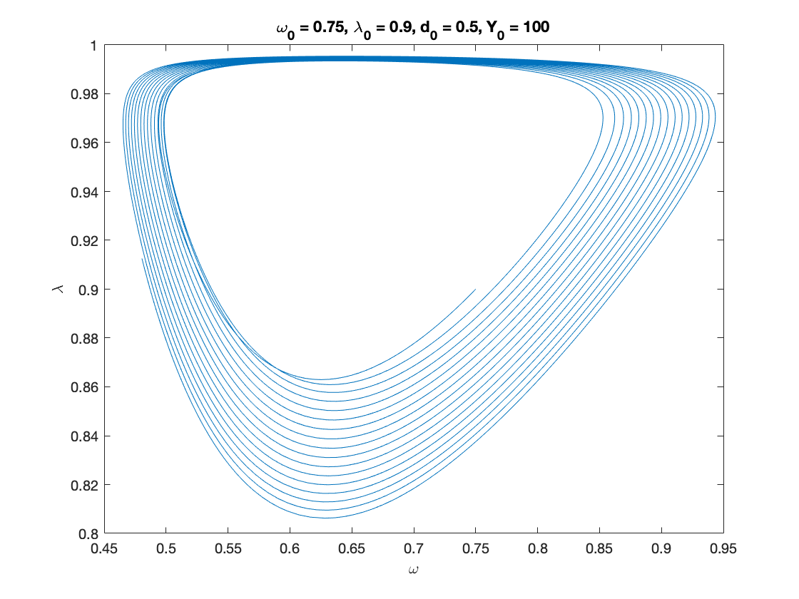
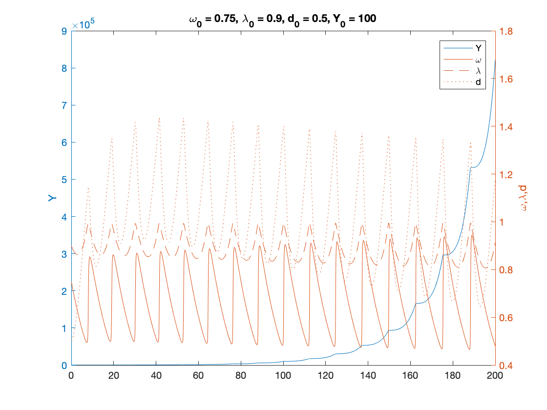
% Parameters as in Table 3 except for eta_p and gamma

nu = 3;         %capital to output ratio
alpha = 0.025;  %productivity growth rate
beta = 0.02;    %population growth rate
delta = 0.05;   %depreciation rate
r = 0.03;       %real interest rate
eta_p = 0.45;   % adjustment speed for prices - MODIFIED
markup = 1.6;   % mark-up value
gamma = .96;    % (1-gamma) is the degree of money ilusion - MODIFIED

% Numerical Values of Interest
c_eq=1-nu*(alpha+beta+delta)
eta_1 = fun_consumption_inv(c_eq)

A_w = eta_p*markup; % Coefficients in the quadratic equation A_w omega^2 + B_w omega + C_w = 0
B_w = alpha+beta-eta_p*(1+eta_1*markup);
C_w = eta_1*(eta_p-alpha-beta)+r*(eta_1-c_eq);

x=[];
syms x
omega_1 = vpasolve(A_w*x^2+B_w*x+C_w ==0,x)
i_omega_1 = eta_p*(markup*omega_1-1)
g_nominal_1 = alpha+beta+i_omega_1
lambda_1 = fun_Phi_inv(alpha+(1-gamma)*eta_p*(markup*omega_1-1))
d_1 = (omega_1-eta_1)./r

eta_1_calc=omega_1-r.*d_1; % verification step
c_eq_calc=fun_consumption(eta_1_calc); %verification step


% Sample paths of the dual Keen model

omega0 = 0.75;
lambda0 = 0.9;
d0 = 0.5;
Y0 = 100;
T = 200;

[tK,yK] = ode15s(@(t,y) dual_keen(y), [0 T], convert([omega0, lambda0, d0]), options);
yK = retrieve(yK);
Y_output = Y0*yK(:,2)/lambda0.*exp((alpha+beta)*tK);

n=length(yK(:,3))

omega_bar = yK(n,1)
lambda_bar = yK(n,2)
d_bar = yK(n,3)

figure(3)
plot(yK(:,1), yK(:,2)), hold on;
%plot(bar_omega_K, bar_lambda_K, 'ro')
xlabel('\omega')
ylabel('\lambda')
title(['\omega_0 = ', num2str(omega0, txt_format), ...
    ', \lambda_0 = ', num2str(lambda0, txt_format), ...
    ', d_0 = ', num2str(d0, txt_format), ...
    ', Y_0 = ', num2str(Y0, txt_format)])
print('dual_keen_phase_cycle','-depsc')

figure(4)
yyaxis right
plot(tK, yK(:,1),tK,yK(:,2),tK,yK(:,3))
ylabel('\omega,\lambda,d')

yyaxis left
plot(tK, Y_output)
ylabel('Y')

title(['\omega_0 = ', num2str(omega0,txt_format), ...
    ', \lambda_0 = ', num2str(lambda0, txt_format), ...
    ', d_0 = ', num2str(d0, txt_format), ...
    ', Y_0 = ', num2str(Y0, txt_format)])
legend('Y','\omega', '\lambda','d')
print('dual_keen_time_cycle','-depsc')
%

c_eq =

    0.7150


eta_1 =

    0.6059

 
omega_1 =
 
 0.51337660572143848603532778591854
 0.65503187710354006988977171337227
 
 
i_omega_1 =
 
 -0.08036884388056429005456399413865
 0.021622951514548850320635633628032
 
 
g_nominal_1 =
 
 -0.03536884388056429005456399413865
 0.066622951514548850320635633628032
 
 
lambda_1 =
 
 0.96780635616165993232539783359532
 0.96881832873512291925191143457792
 
 
d_1 =
 
 -3.0843959034513356629923904457422
  1.6374464759520504654890738027153
 

n =

        4963


omega_bar =

    0.4805


lambda_bar =

    0.9126


d_bar =

    1.1803

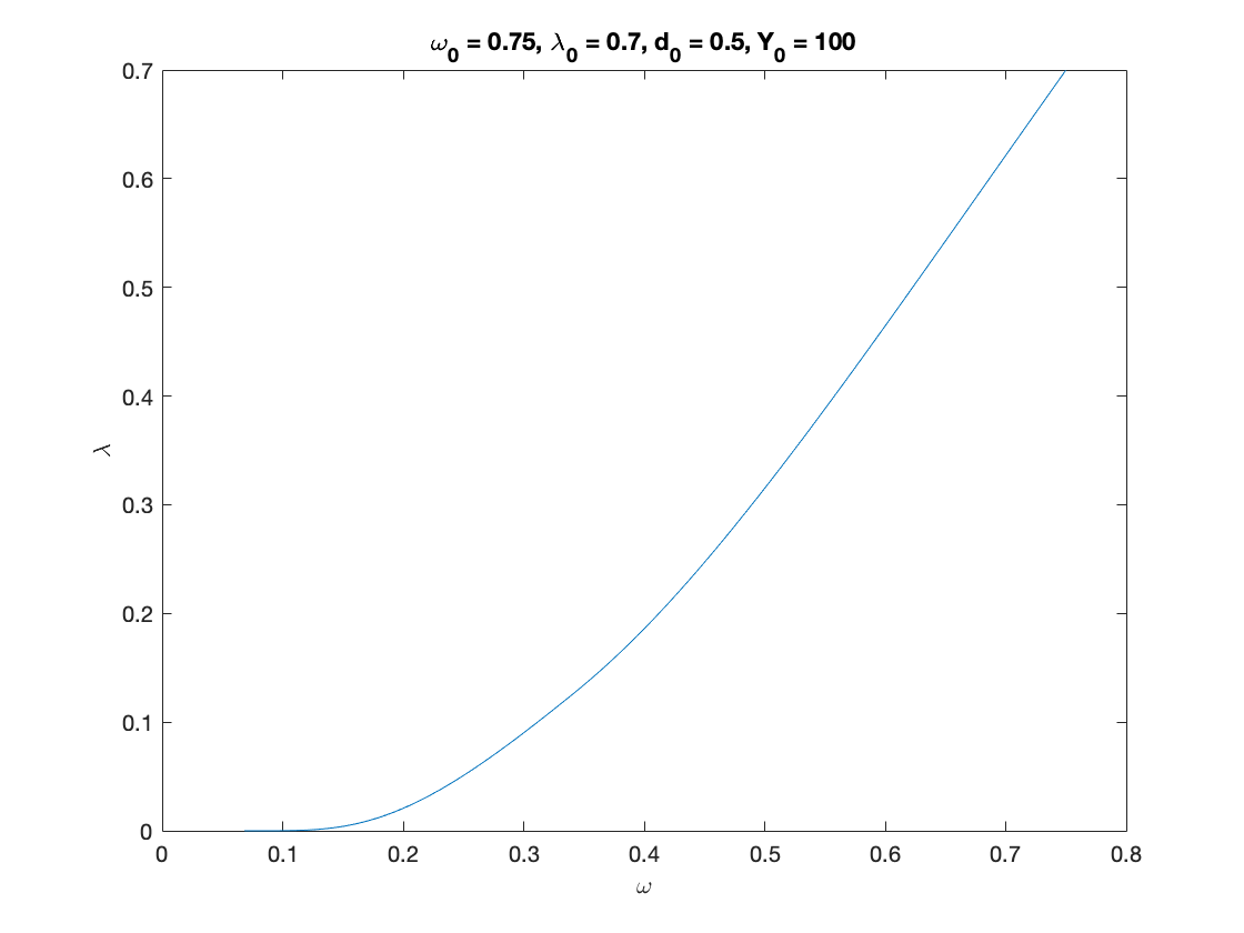
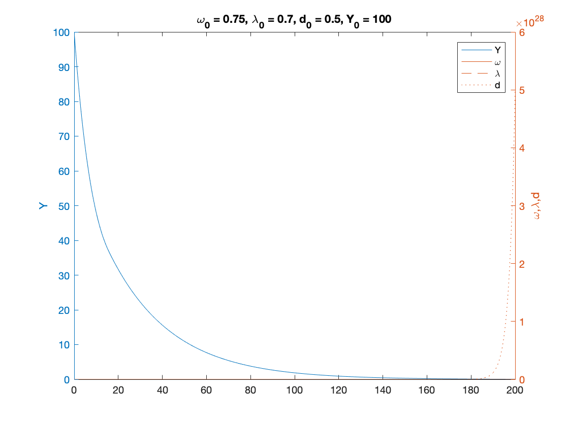
Example 3

Parameters as in Table 3 except for nu AND delta

nu = 15;          % capital to output ratio - MODIFIED
alpha = 0.025;    % productivity growth rate
beta = 0.02;      % population growth rate
delta = 0.10;     % depreciation rate - MODIFIED (NOTE: this is 0.05 in the paper)
r = 0.03;         % real interest rate
eta_p = 0.35;     % adjustment speed for prices
markup = 1.6;     % mark-up value
gamma = 0.8;      % (1-gamma) is the degree of money ilusion


% Numerical Values of Interest
c_eq=1-nu*(alpha+beta+delta)
eta_1 = fun_consumption_inv(c_eq)

A_w = eta_p*markup; % Coefficients in the quadratic equation A_w omega^2 + B_w omega + C_w = 0
B_w = alpha+beta-eta_p*(1+eta_1*markup);
C_w = eta_1*(eta_p-alpha-beta)+r*(eta_1-c_eq);

x=[];
syms x
omega_1 = vpasolve(A_w*x^2+B_w*x+C_w ==0,x)
i_omega_1 = eta_p*(markup*omega_1-1)
g_nominal_1 = alpha+beta+i_omega_1
lambda_1 = fun_Phi_inv(alpha+(1-gamma)*eta_p*(markup*omega_1-1))
d_1 = (omega_1-eta_1)./r

eta_1_calc=omega_1-r.*d_1; % verification step
c_eq_calc=fun_consumption(eta_1_calc); %verification step

% Sample paths of the dual Keen model

omega0 = 0.75;
lambda0 = 0.7;
d0 = 0.5;
Y0 = 100;
T = 200;

[tK,yK] = ode15s(@(t,y) dual_keen(y), [0 T], convert([omega0, lambda0, d0]), options);
yK = retrieve(yK);
Y_output = Y0*yK(:,2)/lambda0.*exp((alpha+beta)*tK);

n=length(yK(:,3))

omega_bar = yK(n,1)
lambda_bar = yK(n,2)
d_bar = yK(n,3)

g_bar=(1-c_minus)/nu-delta

figure(5)
plot(yK(:,1), yK(:,2)), hold on;
%plot(bar_omega_K, bar_lambda_K, 'ro')
xlabel('\omega')
ylabel('\lambda')
title(['\omega_0 = ', num2str(omega0, txt_format), ...
    ', \lambda_0 = ', num2str(lambda0, txt_format), ...
    ', d_0 = ', num2str(d0, txt_format), ...
    ', Y_0 = ', num2str(Y0, txt_format)])
print('dual_keen_phase_divergent','-depsc')


figure(6)
yyaxis right
plot(tK, yK(:,1),tK,yK(:,2),tK,yK(:,3))
ylabel('\omega,\lambda,d')

yyaxis left
plot(tK, Y_output)
ylabel('Y')



title(['\omega_0 = ', num2str(omega0,txt_format), ...
    ', \lambda_0 = ', num2str(lambda0, txt_format), ...
    ', d_0 = ', num2str(d0, txt_format), ...
    ', Y_0 = ', num2str(Y0, txt_format)])
legend('Y','\omega', '\lambda','d')
print('dual_keen_time_divergent','-depsc')
%

c_eq =

   -1.1750


eta_1 =

   0.0956 - 0.3934i

 
omega_1 =
 
  0.1375268793268625106771715577569 - 0.49617911095986802963355036671393i
 0.50275218583166006178002563156168 + 0.10281657191707506091722022599555i
 
 
i_omega_1 =
 
   - 0.27298494757695699402078392765613 - 0.2778603021375260965947882053598i
 - 0.06845877593427036540318564632546 + 0.057577280273562034113643326557506i
 
 
g_nominal_1 =
 
   - 0.22798494757695699402078392765613 - 0.2778603021375260965947882053598i
 - 0.02345877593427036540318564632546 + 0.057577280273562034113643326557506i
 
 
lambda_1 =
 
  0.97408289957607732385023306587867 - 0.021491278192165304543281057486094i
 0.96531792041637275646895074345848 + 0.0038394716601090056851942825208078i
 
 
d_1 =
 
 1.3963557103732356393956844389596 - 3.4272190639025027575057498472755i
 13.570532593866487342824153565785 + 16.539303698662266927519936576374i
 

n =

   830


omega_bar =

    0.0683


lambda_bar =

   4.7264e-08


d_bar =

   5.0107e+28


g_bar =

   -0.0353

Auxiliary functions

Instead of integrating the system in terms of omega, lambda and d, we decided to use:

log_omega = log(omega), tan_lambda = tan((lambda-0.5)*pi), and y_h=omega-r*d disposable income of households

Experiments show that the numerical methods work better with these variables.

function new = convert(old)
    % This function converts
    % [omega, lambda, d, p]
    % to
    % [log_omega, tan_lambda, y]
    % It also work with the first 2 components alone.
    % each of these variables might also be a time-dependent vector

    n = size(old,2); %number of variables
    new = zeros(size(old));

    new(:,1) = log(old(:,1));
    new(:,2) = tan((old(:,2)-0.5)*pi);
    if n>2
        new(:,3) = old(:,1)-r.*old(:,3);
    end
end

function old = retrieve(new)
    % This function retrieves [omega, lambda, d, p]
    % from
    % [log_omega, tan_lambda, pi_n, log_p]
    %
    %  It also work with the first 2 or 3 elements alone.
    % each of these variables might also be a time-dependent vector

    n = size(new,2); %number of variables
    old = zeros(size(new));

    old(:,1) = exp(new(:,1));
    old(:,2) = atan(new(:,2))/pi+0.5;
    if n>2
        old(:,3) = (old(:,1)-new(:,3))./r;
    end
end


function f = dual_keen(y)
    f = zeros(3,1);
    log_omega = y(1);
    tan_lambda = y(2);
    y_h = y(3);
    lambda = atan(tan_lambda)/pi+0.5;
    omega = exp(log_omega);
    g_Y = (1-fun_consumption(y_h))./nu-delta;

    f(1) = fun_Phi(lambda)-alpha-(1-gamma)*eta_p*(markup*omega-1); %d(log_omega)/dt
    f(2) = (1+tan_lambda^2)*pi*lambda*(g_Y-alpha-beta); %d(tan_lambda)/dt
    f(3) = omega*f(1)-r*(fun_consumption(y_h)-y_h)+(omega-y_h)*(g_Y+eta_p*(markup*omega-1)); %d(y_h)/dt
end

end