Contents

function out = goodwin()

%%%%%%%%%%%%%%%%%%%%%%%%%%%%%%%%%%%%%%%%%%%%%%%%%%%%%%%%%%%%%%%%%%%%%%%%%%%
% This code simulates the Goodwin model as specified in Grasselli and Costa Lima (2012).
%
% authors: B. Costa Lima and M. Grasselli
%%%%%%%%%%%%%%%%%%%%%%%%%%%%%%%%%%%%%%%%%%%%%%%%%%%%%%%%%%%%%%%%%%%%%%%%%%%
close all
clc
warning off

Parameters attribution

Equations (24) and (26)

nu = 3;              % capital-to-output ratio
alpha = 0.025;       % productivity growth rate
beta = 0.02;         % population growth rate
delta = 0.01;        % depreciation rate
phi0 = 0.04/(1-0.04^2); %Phillips curve parameter,  Phi(0.96)=0
phi1 = 0.04^3/(1-0.04^2); %Phillips curve parameter, Phi(0)=-0.04

Other definitions

TOL = 1E-7;
options = odeset('RelTol', TOL);
txt_format = '%3.3g';

Functions Definition

fun_Phi = @(x) phi1./(1-x).^2- phi0;           % Phillips curve, equation (25)
fun_Phi_prime = @(x) 2*phi1./(1-x).^3;         % derivative of Phillips curve
fun_Phi_inv = @(x) 1 - (phi1/(x+phi0)).^(1/2); % inverse of Phillips curve

Numerical values of interest

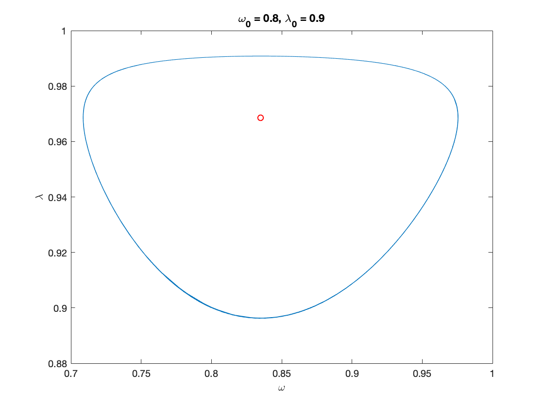
omega_bar =  1-nu*(alpha+beta+delta)           % equilibrium wage share, equation (27)
lambda_bar = fun_Phi_inv(alpha)                % equilibrium employment rate, equation (27)

omega_bar =

    0.8350


lambda_bar =

    0.9686

Sample paths of the Goodwin model

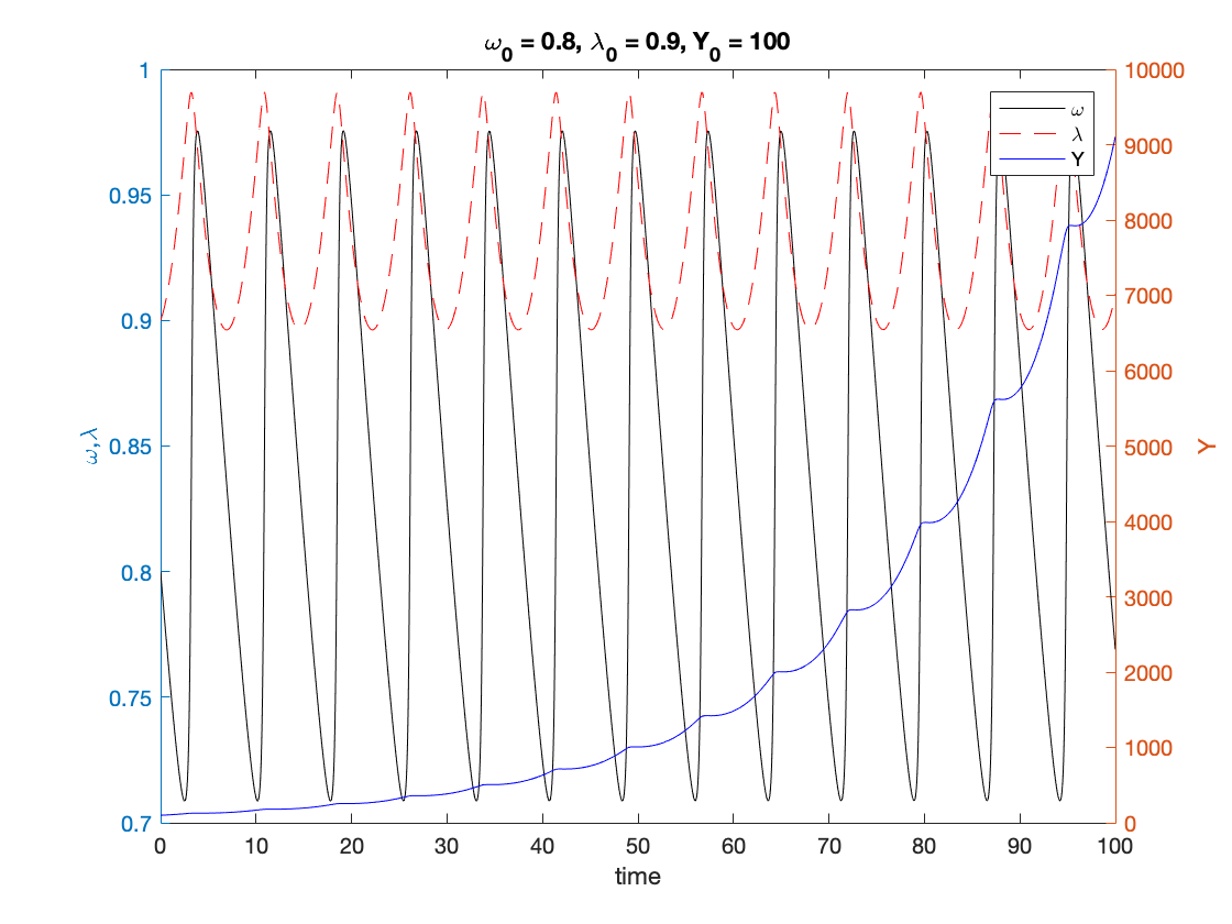
omega0 = 0.80;                                 % initial wage share
lambda0 = 0.90;                                % initial employment rate
Y0 = 100;                                      % initial GDP
T = 100;                                       % time in years

[tG,yG] = ode15s(@(t,y) goodwin(y), [0 T], [omega0, lambda0], options);
Y_output = Y0*yG(:,2)/lambda0.*exp((alpha+beta)*tG);        % Y(t)=a(t)*L(t), equation (5)

% Figure 1
figure(1)
plot(yG(:,1), yG(:,2)), hold on;
plot(omega_bar, lambda_bar, 'ro')
xlabel('\omega')
ylabel('\lambda')
title(['\omega_0 = ', num2str(omega0, txt_format), ...
    ', \lambda_0 = ', num2str(lambda0, txt_format)])
print('goodwin_phase','-depsc')

% Figure 2
figure(2)
yyaxis left
plot(tG, yG(:,1), 'k', tG, yG(:,2), 'r')
ylabel('\omega,\lambda')

yyaxis right
plot(tG,Y_output, 'b')
ylabel('Y')

xlabel('time')


title(['\omega_0 = ', num2str(omega0,txt_format), ...
    ', \lambda_0 = ', num2str(lambda0, txt_format), ...
    ', Y_0 = ', num2str(Y0, txt_format)])
legend('\omega', '\lambda', 'Y')
print('goodwin_time','-depsc')

Auxiliary functions

function f = goodwin(y)
    f = zeros(2,1);
    omega = y(1);
    lambda = y(2);

    % Equation (12)
    f(1) = omega*(fun_Phi(lambda)-alpha);                 % d(omega)/dt
    f(2) = lambda*((1-omega)/nu-alpha-beta-delta);        % d(lambda)/dt
end

end

Published with MATLAB® R2017a