Contents

function out = inflation_paper()

%%%%%%%%%%%%%%%%%%%%%%%%%%%%%%%%%%%%%%%%%%%%%%%%%%%%%%%%%%%%%%%%%%%%%%%%%%%
% This code simulates the Keen model with inflation as
% specified in Grasselli and Nguyen Huu (2015)
%
% authors: M. Grasselli and A. Nguyen Huu
%%%%%%%%%%%%%%%%%%%%%%%%%%%%%%%%%%%%%%%%%%%%%%%%%%%%%%%%%%%%%%%%%%%%%%%%%%%
close all
clc
warning off

Base Parameters

Equations (76),(77)

phi0 = 0.0401;       %Phillips curve parameter
phi1 = 6.41e-05;     %Phillips curve parameter

kappa0 = -0.0065;    % constant parameter in investment function
kappa1 = -5;         % affine parameter in exponent of investment function
kappa2 = 20;         % coefficient in the exponent of investment function

psi0 = 0.25;         % parameter for speculation function
psi1 = 0.02;         % parameter for speculation function
psi2 = 1.2;          % parameter for speculation function

Other definitions

TOL = 1E-7;
options = odeset('RelTol', TOL);
txt_format = '%3.3g';

Functions of interest

inflation = @(x) eta_p*(markup*x-1);                                       % inflation, equation (2.64)

phillips = @(x) phi1./(1-x).^2- phi0;                                       % Phillips curve, equation (76)
phillips_prime = @(x) 2*phi1./(1-x).^3;                                     % derivative of phillips curve
phillips_inv = @(x) 1 - (phi1./(x+phi0)).^(1/2);                            % inverse of phillips curve

investment= @(x) kappa0+exp(kappa1+kappa2.*x);                 % investment function, equation (25)
investment_prime= @(x) kappa2.*exp(kappa1+kappa2.*x);          % derivative of investment function
investment_inv= @(x) (log(x-kappa0)-kappa1)./kappa2;           % inverse of investment function

speculation=@(x) psi0.*(exp(psi2.*(x-psi1))-1);                % speculation function, equation (83)

Section 5.1.1 - Basic Keen model

% Equation (75)
alpha = 0.025;       % productivity growth rate
beta = 0.02;         % population growth rate
delta = 0.01;        % depreciation rate
nu = 3;              % capital to output ratio
r = 0.03;             % interest rate on loans

pi_eq=investment_inv(nu*(alpha+beta+delta))       % profit share at interior equilibrium, equations (16) and (78)
b_eq=(investment(pi_eq)-pi_eq)/(alpha+beta);      % debt level at equilibrium, equation (19)
lambda_eq=phillips_inv(alpha);                    % employment at equilibirum, equation (18)
omega_eq=1-pi_eq-r*b_eq;                         % wage share at equilibrium, equation (17)

eq1 =[omega_eq,lambda_eq,b_eq]

pi_eq =

    0.1618


eq1 =

    0.8361    0.9686    0.0702

Section 5.1.2 - Keen Model with inflation

% Equation (75)
alpha = 0.025;       % productivity growth rate
beta = 0.02;         % population growth rate
delta = 0.01;        % depreciation rate
nu = 3;              % capital to output ratio
r = 0.03;             % interest rate on loans

% Additional parameters, equation (79)
eta_p = 4;            % adjustment speed for prices
markup = 1.2;        % mark-up value
gamma = 0.8;         % inflation sensitivity in the bargaining equation

% Coefficients for quadratic for omega, equations before (30)
a0=markup*eta_p;
a1=alpha+beta-eta_p*(1+markup*(1-pi_eq));
a2=(eta_p-alpha-beta)*(1-pi_eq)+r*(investment(pi_eq)-pi_eq);
a=[a0,a1,a2];

% Solve quadratic equation for omega
omega_eq = roots(a);

% Find interior equilibrium employment and debt, equations (28) and (29)
inflation = @(x) eta_p*(markup*x-1);
lambda_eq = phillips_inv(alpha+(1-gamma)*inflation(omega_eq));
b_eq=(investment(pi_eq)-pi_eq)./(alpha+beta+inflation(omega_eq));

% Display result, equation (81)
eq1_plus=[omega_eq(1),lambda_eq(1),b_eq(1)]
eq1_minus=[omega_eq(2),lambda_eq(2),b_eq(2)]
inflation_eq = inflation(omega_eq)

% % Compute omega3 using (33)
% Something is wrong here: there is no solution for b3
% omega3=1/markup+(phillips(0)-alpha)/(markup*eta_p*(1-gamma))
% i3=inflation(omega3)
%
% % Compute b3 using (34)
% b=[];
% syms b
% eqn1=b*(i3+investment(1-omega3-r*b)/nu-delta-r);
% eqn2=investment(1-omega3-r*b)-1+omega3;
% b3=vpasolve(eqn1==eqn2,b)

eq1_plus =

    0.8366    0.9693    0.0521


eq1_minus =

    0.8255    0.9666    0.4213


inflation_eq =

    0.0157
   -0.0375

Section 5.1.3 - Keen Model with Inflation and Speculation

eta_p = 4;           % adjustment speed for prices
markup = 1.2;        % mark-up value
gamma = 0.8;         % inflation sensitivity in the bargaining equation
inflation = @(x) eta_p*(markup*x-1);

% Additional parameters, equation before (83)
rL= 0.03;           % interest rate on loans
rf= 0.028;          % interest rate on deposits

% Coefficients for the nonlinear equation for X, equation (62)
v1=eta_p*markup*(pi_eq-1)-alpha-beta+eta_p;
v2=eta_p*markup*(rL*investment(pi_eq)-rf*pi_eq);
v3=(rL-rf)*eta_p*markup;

% Solve equation (62)
z=[];
syms z
x=vpasolve(z^3+v1*z^2+v2*z+v3*speculation(z)==0,z);
X=double(x);
i_eq=X-alpha-beta

% Find equilibirum values, equations (58)-(61)
f_eq=speculation(X)/X;
c_eq=(rL*investment(pi_eq)-rf*pi_eq+(rL-rf)*f_eq)/X;
lambda_eq=phillips_inv(alpha-(1-gamma)*i_eq);
omega_eq=1-pi_eq-c_eq;

% Display equilibrium values, equation (84)
% NOTE: these are slightly different from the values
% shown in the paper, probably because some parameter is wrong
eq1=[omega_eq,lambda_eq,c_eq,f_eq]
inflation_eq=inflation(omega_eq)

i_eq =

   -0.0311


eq1 =

    0.8269    0.9700    0.0113   -0.1306


inflation_eq =

   -0.0311

Section 5.2.1 - Keen Model with Inflation (Dynamics)

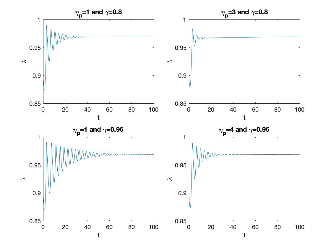
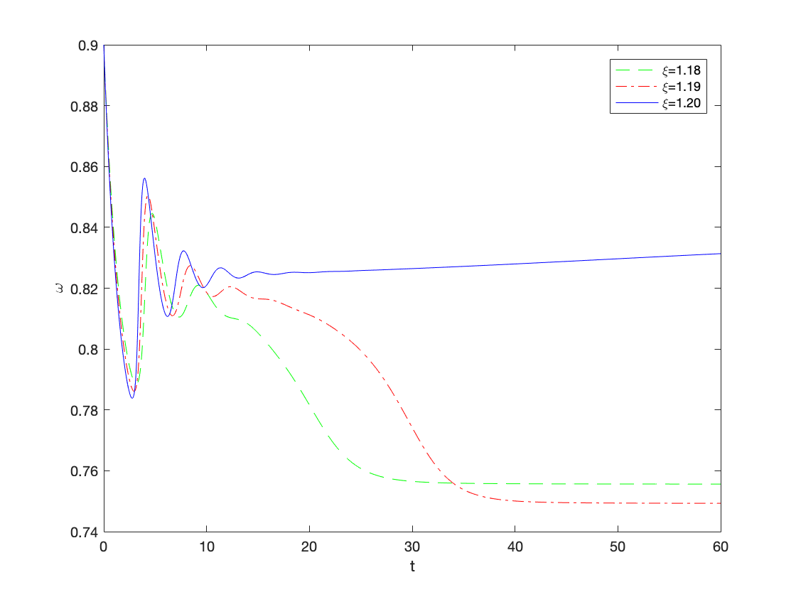
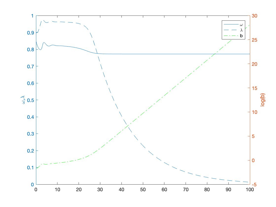
alpha = 0.025;       % productivity growth rate
beta = 0.02;         % population growth rate
delta = 0.01;        % depreciation rate
nu = 3;              % capital to output ratio
r = 0.03;             % interest rate on loans

% Figure 1
figure(1)

omega0=0.9;
lambda0=0.9;
b0=0.3;
T=100;

subplot(2,2,1)
eta_p=1;
gamma=0.8;
markup=1.20;
inflation = @(x) eta_p*(markup*x-1);
y0=[convert([omega0,lambda0]),b0];
[tK,yK] = ode15s(@(t,y) keen_inflation(y), [0 T], y0, options);
sol = retrieve([yK(:,1),yK(:,2)]);
yK(:,1)=sol(:,1);
yK(:,2)=sol(:,2);
plot(tK,yK(:,2))
title('\eta_p=1 and \gamma=0.8')
xlabel('t')
ylabel('\lambda')

subplot(2,2,2)
eta_p=3;            % NOTE: with eta_p=4 as in the paper, lambda collapses to zero!
gamma=0.8;
markup=1.20;
inflation = @(x) eta_p*(markup*x-1);
y0=[convert([omega0,lambda0]),b0];
[tK,yK] = ode15s(@(t,y) keen_inflation(y), [0 T], y0, options);
sol = retrieve([yK(:,1),yK(:,2)]);
yK(:,1)=sol(:,1);
yK(:,2)=sol(:,2);
plot(tK,yK(:,2))
title('\eta_p=3 and \gamma=0.8')
xlabel('t')
ylabel('\lambda')

subplot(2,2,3)
eta_p=1;
gamma=0.96;
markup=1.20;
inflation = @(x) eta_p*(markup*x-1);
y0=[convert([omega0,lambda0]),b0];
[tK,yK] = ode15s(@(t,y) keen_inflation(y), [0 T], y0, options);
sol = retrieve([yK(:,1),yK(:,2)]);
yK(:,1)=sol(:,1);
yK(:,2)=sol(:,2);
plot(tK,yK(:,2))
title('\eta_p=1 and \gamma=0.96')
xlabel('t')
ylabel('\lambda')

subplot(2,2,4)
eta_p=4;
gamma=0.96;
markup=1.20;
inflation = @(x) eta_p*(markup*x-1);
y0=[convert([omega0,lambda0]),b0];
[tK,yK] = ode15s(@(t,y) keen_inflation(y), [0 T], y0, options);
sol = retrieve([yK(:,1),yK(:,2)]);
yK(:,1)=sol(:,1);
yK(:,2)=sol(:,2);
plot(tK,yK(:,2))
title('\eta_p=4 and \gamma=0.96')
xlabel('t')
ylabel('\lambda')

% Figure 2
figure(2)
omega0=0.9;
lambda0=0.9;
b0=0.3;
T=60;
y0=[convert([omega0,lambda0]),b0];
eta_p=3;             % NOTE: with eta_p=4 as in the paper, all omegas collapse to zero!
gamma=0.8;

markup=1.18;
inflation = @(x) eta_p*(markup*x-1);
[tK1,yK1] = ode15s(@(t,y) keen_inflation(y), [0 T], y0, options);
sol = retrieve([yK1(:,1),yK1(:,2)]);
yK1(:,1)=sol(:,1);
yK1(:,2)=sol(:,2);

markup=1.19;
inflation = @(x) eta_p*(markup*x-1);
[tK2,yK2] = ode15s(@(t,y) keen_inflation(y), [0 T], y0, options);
sol = retrieve([yK2(:,1),yK2(:,2)]);
yK2(:,1)=sol(:,1);
yK2(:,2)=sol(:,2);

markup=1.20;
inflation = @(x) eta_p*(markup*x-1);
[tK3,yK3] = ode15s(@(t,y) keen_inflation(y), [0 T], y0, options);
sol = retrieve([yK3(:,1),yK3(:,2)]);
yK3(:,1)=sol(:,1);
yK3(:,2)=sol(:,2);

plot(tK1,yK1(:,1),'--g')
hold on
plot(tK2,yK2(:,1),'-.r')
plot(tK3,yK3(:,1),'-b')
legend('\xi=1.18','\xi=1.19','\xi=1.20')
xlabel('t')
ylabel('\omega')

% Figure 3
figure(3)

omega0=0.85;
lambda0=0.9;
b0=0.2;
T=100;
y0=[convert([omega0,lambda0]),b0];

eta_p=4;
gamma=0.8;
markup=1.19;                           % NOTE: with markup=1.20 as in the paper, the system converges to the interior equilibrium
inflation = @(x) eta_p*(markup*x-1);

[tK,yK] = ode15s(@(t,y) keen_inflation(y), [0 T], y0, options);
sol = retrieve([yK(:,1),yK(:,2)]);
yK(:,1)=sol(:,1);
yK(:,2)=sol(:,2);

yyaxis left
plot(tK,yK(:,1),'-',tK,yK(:,2),'--')
ylabel('\omega,\lambda')

yyaxis right
plot(tK,log(yK(:,3)),'-.g')
ylabel('log(b)')
legend('\omega','\lambda','b')

Section 5.2.2 - Keen Model with Inflation and Speculation (Dynamics)

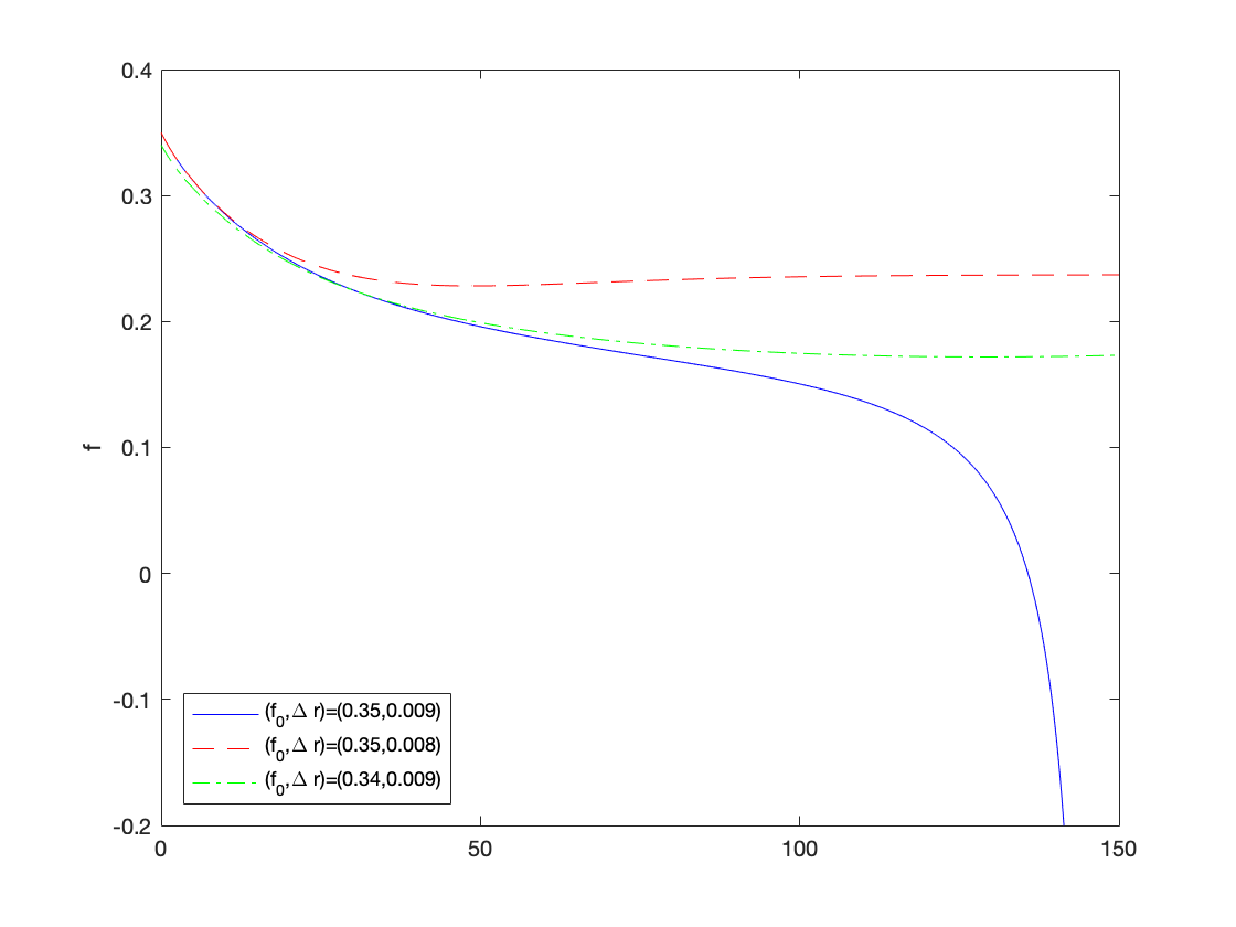
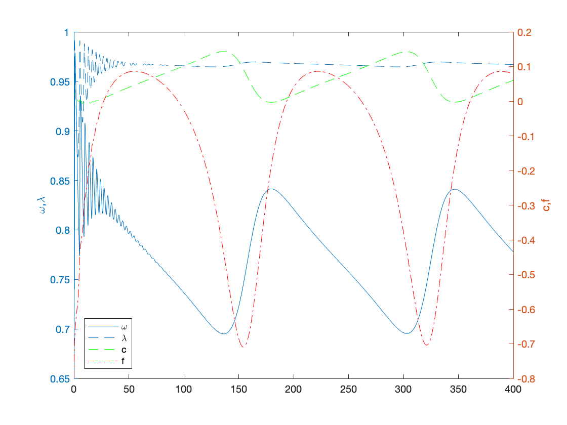
% Figure 4
figure(4)

omega0=0.9;
lambda0=0.9;
c0=0.05;
T=150;

eta_p=1;
gamma=0.8;
markup=1.3;
inflation = @(x) eta_p*(markup*x-1);

f0=0.35;
rf=0.02;                % NOTE: it is unclear what the choice of rL and rf is at this point in the paper
rL=rf+0.009;            % but the difference should be \Delta r = 0.009 instead of 0.09

y0=[convert([omega0,lambda0]),c0,f0];
[tK,yK] = ode15s(@(t,y) main(y), [0 T], y0, options);
sol = retrieve([yK(:,1),yK(:,2)]);
yK(:,1)=sol(:,1);
yK(:,2)=sol(:,2);

plot(tK,yK(:,4),'b')
ylabel('f')
ylim([-0.2,0.4])
hold on


f0=0.35;
rf=0.02;
rL=rf+0.008;

y0=[convert([omega0,lambda0]),c0,f0];
[tK,yK] = ode15s(@(t,y) main(y), [0 T], y0, options);
sol = retrieve([yK(:,1),yK(:,2)]);
yK(:,1)=sol(:,1);
yK(:,2)=sol(:,2);

plot(tK,yK(:,4),'--r')
ylabel('f')
hold on


f0=0.34;
rf=0.02;
rL=rf+0.009;

y0=[convert([omega0,lambda0]),c0,f0];
[tK,yK] = ode15s(@(t,y) main(y), [0 T], y0, options);
sol = retrieve([yK(:,1),yK(:,2)]);
yK(:,1)=sol(:,1);
yK(:,2)=sol(:,2);

plot(tK,yK(:,4),'-.g')
ylabel('f')
legend('(f_0,\Delta r)=(0.35,0.009)','(f_0,\Delta r)=(0.35,0.008)','(f_0,\Delta r)=(0.34,0.009)','Location','SouthWest')



% Figure 5
figure(5)
omega0=0.75;
lambda0=0.9;
c0=0.02;
f0=-0.8;
T=400;
y0=[convert([omega0,lambda0]),c0,f0];
rL=0.03;
rf=0.02;
eta_p=0.4;
gamma=0.8;
markup=1.21;
inflation = @(x) eta_p*(markup*x-1);

[tK,yK] = ode15s(@(t,y) main(y), [0 T], y0, options);
sol = retrieve([yK(:,1),yK(:,2)]);
yK(:,1)=sol(:,1);
yK(:,2)=sol(:,2);

yyaxis left
ylim([0.65,1])
plot(tK,yK(:,1),'-',tK,yK(:,2),'--')
ylabel('\omega,\lambda')

yyaxis right
ylim([-0.8,0.5])
plot(tK,yK(:,3),'--g',tK,yK(:,4),'-.r')
ylabel('c,f')
legend('\omega','\lambda','c','f','Location','SouthWest')


function new = convert(old)
    % This function converts
    % [omega, lambda]
    % to
    % [log_omega, tan_lambda]


    n = size(old,2); %number of variables
    new = zeros(size(old));

    new(:,1) = log(old(:,1));
    new(:,2) = tan((old(:,2)-0.5)*pi);
end

function old = retrieve(new)
    % This function retrieves [omega, lambda]
    % from
    % [log_omega, tan_lambda]

    n = size(new,2); %number of variables
    old = zeros(size(new));

    old(:,1) = exp(new(:,1));
    old(:,2) = atan(new(:,2))/pi+0.5;
end

function f = keen_inflation(y)    % solves the Keen model with inflation
    f = zeros(3,1);

    log_omega = y(1);
    tan_lambda = y(2);
    b = y(3);

    lambda = atan(tan_lambda)/pi+0.5;
    omega = exp(log_omega);
    profit = 1-omega-r*b;

    growth = investment(profit)/nu-delta;    % real growth rate

    % Equation (57)
    f(1) = phillips(lambda)-(1-gamma)*inflation(omega)-alpha; %d(log_omega)/dt
    f(2) = (1+tan_lambda^2)*pi*lambda*(growth-alpha-beta); %d(tan_lambda)/dt
    f(3) = investment(profit)-profit-(growth+inflation(omega))*b; %db/dt

end


function f = main(y)    % solves the main dynamical system
    f = zeros(4,1);

    log_omega = y(1);
    tan_lambda = y(2);
    c = y(3);
    F= y(4);

    lambda = atan(tan_lambda)/pi+0.5;
    omega = exp(log_omega);
    profit = 1-omega-c;

    growth = investment(profit)/nu-delta;    % real growth rate

    % Equation (57)
    f(1) = phillips(lambda)-(1-gamma)*inflation(omega)-alpha; %d(log_omega)/dt
    f(2) = (1+tan_lambda^2)*pi*lambda*(growth-alpha-beta); %d(tan_lambda)/dt
    f(3) = rL*investment(profit)-rf*profit-(growth+inflation(omega))*c+(rL-rf)*F; %dc/dt
    f(4) = speculation(growth+inflation(omega))-(growth+inflation(omega))*F;   %dF/dt

end

end

Published with MATLAB® R2017a