Contents

function out = inventories()

%%%%%%%%%%%%%%%%%%%%%%%%%%%%%%%%%%%%%%%%%%%%%%%%%%%%%%%%%%%%%%%%%%%%%%%%%%%
% This code simulates the Inventory Model as specified in
% Grasselli and Nguyen-Huu (2018)
%
%
% authors: M. Grasselli and A. Nguyen-Huu
%%%%%%%%%%%%%%%%%%%%%%%%%%%%%%%%%%%%%%%%%%%%%%%%%%%%%%%%%%%%%%%%%%%%%%%%%%%
clear all
close all
clc
warning off

Base Parameters

This is a combination of Grasselli and Nguyen-Huu (2015) and Giraud and Grasselli (2019)

phi0 = 0.0401;       %Phillips curve parameter
phi1 = 6.41e-05;     %Phillips curve parameter

kappa0 = -0.0065;    % constant parameter in investment function
kappa1 = -5;         % affine parameter in exponent of investment function
kappa2 = 20;         % coefficient in the exponent of investment function
eta_u = 0.2;        % adjustment speed for investment as function of utilization
u_b = 0.9;           % baseline utilization

c_minus= 0.03; % consumption share hard-lower bound
A_c = 0; %Consumption share asymptotic lower bound
B_c = 5; % Consumption share growth rate
C_c = 1;
K_c = 0.9; %Consumption share upper bound
nu_c = 0.2;
Q_c= ((K_c-A_c)/(c_minus-A_c))^nu_c-C_c;

Other definitions

TOL = 1E-7;
options = odeset('RelTol', TOL);
txt_format = '%3.3g';

Functions of interest

inflation = @(x1,x2,x3) eta_p*(markup*x1-1)+eta_q*(x2-x3);    % inflation, equation (31)

phillips = @(x) phi1./(1-x).^2- phi0;                         % Phillips curve, equation (32)
phillips_prime = @(x) 2*phi1./(1-x).^3;                       % derivative of phillips curve
phillips_inv = @(x) 1 - (phi1./(x+phi0)).^(1/2);              % inverse of phillips curve

investment= @(x1,x2) kappa0+exp(kappa1+kappa2.*x1)+eta_u*(x2-u_b); % investment function, equation (25)

% consumption, equation (24) with generalised logistic function depending
% on income only
consumption =@(x) max(c_minus,A_c + ((K_c-A_c)./(C_c+Q_c*exp(-B_c*x)).^(1/nu_c)));
consumption_inv = @(x) -log((((K_c-A_c)./(x-A_c)).^nu_c-C_c)./Q_c)./B_c; % inverse of the consumption function over positive income

Example 1

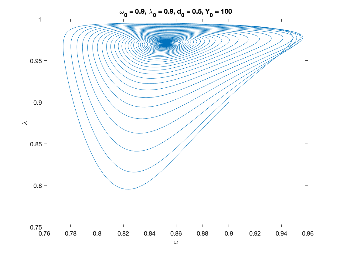
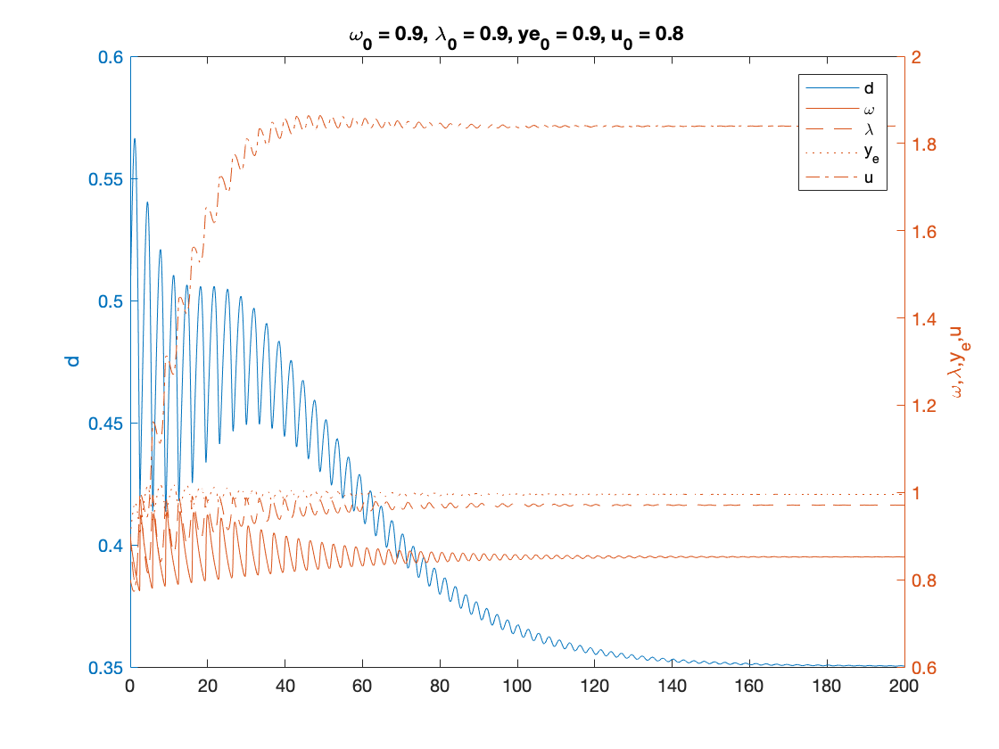
nu = 3;          % capital to output ratio
alpha = 0.025;   % productivity growth rate
beta = 0.02;     % population growth rate
delta = 0.05;    % depreciation rate
r = 0.03;        % real interest rate
eta_p = 0.8;     % adjustment speed for prices with respect to cost
eta_q = 0.2;     % adjustment speed for prices with respect to demand
eta_e = 0.8;     % adjustment speed for expected sales
eta_d = 0.7;     % adjustment speed for desired inventory
markup = 1.2;    % mark-up value
gamma = 0.4;     % (1-gamma) is the degree of money illusion
f_d = 0.1;       % desired inventories as a fraction of expected sales

% Functions of interest

inflation = @(x1,x2,x3) eta_p*(markup*x1-1)+eta_q*(x2-x3);    % inflation, equation (31)

phillips = @(x) phi1./(1-x).^2- phi0;                         % Phillips curve, equation (32)
phillips_prime = @(x) 2*phi1./(1-x).^3;                       % derivative of phillips curve
phillips_inv = @(x) 1 - (phi1./(x+phi0)).^(1/2);              % inverse of phillips curve

investment= @(x1,x2) kappa0+exp(kappa1+kappa2.*x1)+eta_u*(x2-u_b); % investment function, equation (25)

% consumption, equation (24) with generalised logistic function depending
% on income only
consumption =@(x) max(c_minus,A_c + ((K_c-A_c)./(C_c+Q_c*exp(-B_c*x)).^(1/nu_c)));
consumption_inv = @(x) -log((((K_c-A_c)./(x-A_c)).^nu_c-C_c)./Q_c)./B_c; % inverse of the consumption function over positive income


% Numerical Values of Interest

ydbar = 1/(1+(alpha+beta)*f_d);
yebar = 1/(1+(alpha+beta)*f_d)

x=fsolve(@system2d, [0.9,0.1]);

omegabar=x(1)
dbar=x(2)

ibar=inflation(omegabar,ydbar,yebar);

ubar=(nu*(alpha+beta+delta)*(1+(alpha+beta)*f_d))/(1-consumption(omegabar)*(1+(alpha+beta)*f_d))

kbar=investment(yebar*(1-omegabar)-r*dbar,ubar);

cbar = consumption(omegabar);

lambdabar = phillips_inv(alpha+(1-gamma)*ibar)


% Sample paths of the Keen model with inventories

omega0 = 0.9;
lambda0 = 0.9;
d0 = 0.5;
ye0 = 0.9;
u0 = 0.8;
y0=[convert([omega0, lambda0]),d0,ye0,u0];

Y0 = 100;
T = 200;

[tK,yK] = ode15s(@(t,y) keen_inventory(y), [0 T], y0, options);
sol = retrieve([yK(:,1),yK(:,2)]);
yK(:,1)=sol(:,1);
yK(:,2)=sol(:,2);
Y_output = Y0*yK(:,2)/lambda0.*exp((alpha+beta)*tK);

n=length(yK(:,3));

omega_eq = yK(n,1)
lambda_eq = yK(n,2)
d_eq = yK(n,3)
ye_eq = yK(n,4)
u_eq = yK(n,5)

figure(1)
plot(yK(:,1), yK(:,2)), hold on;
%plot(bar_omega_K, bar_lambda_K, 'ro')
xlabel('\omega')
ylabel('\lambda')
title(['\omega_0 = ', num2str(omega0, txt_format), ...
    ', \lambda_0 = ', num2str(lambda0, txt_format), ...
    ', d_0 = ', num2str(d0, txt_format), ...
    ', Y_0 = ', num2str(Y0, txt_format)])

% print('dual_keen_phase_convergent','-depsc')

figure(2)
yyaxis right
plot(tK, yK(:,1),tK,yK(:,2),tK,yK(:,4),tK,yK(:,5))
ylabel('\omega,\lambda,y_e,u')

yyaxis left
plot(tK, yK(:,3))
ylabel('d')

title(['\omega_0 = ', num2str(omega0,txt_format), ...
    ', \lambda_0 = ', num2str(lambda0, txt_format), ...
    ', ye_0 = ', num2str(ye0, txt_format), ...
    ', u_0 = ', num2str(u0, txt_format)])
legend('d','\omega', '\lambda','y_e','u')

% print('dual_keen_time_convergent','-depsc')

yebar =

    0.9955


Equation solved.

fsolve completed because the vector of function values is near zero
as measured by the default value of the function tolerance, and
the problem appears regular as measured by the gradient.




omegabar =

    0.8522


dbar =

    0.3503


ubar =

    1.8399


lambdabar =

    0.9710


omega_eq =

    0.8521


lambda_eq =

    0.9710


d_eq =

    0.3503


ye_eq =

    0.9955


u_eq =

    1.8399

Auxiliary functions

Instead of integrating the system in terms of omega, lambda and d, we decided to use:

log_omega = log(omega), tan_lambda = tan((lambda-0.5)*pi), and y_h=omega-r*d disposable income of households

Experiments show that the numerical methods work better with these variables.

function new = convert(old)
    % This function converts
    % [omega, lambda, d, p]
    % to
    % [log_omega, tan_lambda, y]
    % It also work with the first 2 components alone.
    % each of these variables might also be a time-dependent vector

    n = size(old,2); %number of variables
    new = zeros(size(old));

    new(:,1) = log(old(:,1));
    new(:,2) = tan((old(:,2)-0.5)*pi);
    if n>2
        new(:,3) = old(:,1)-r.*old(:,3);
    end
end

function old = retrieve(new)
    % This function retrieves [omega, lambda, d, p]
    % from
    % [log_omega, tan_lambda, pi_n, log_p]
    %
    %  It also work with the first 2 or 3 elements alone.
    % each of these variables might also be a time-dependent vector

    n = size(new,2); %number of variables
    old = zeros(size(new));

    old(:,1) = exp(new(:,1));
    old(:,2) = atan(new(:,2))/pi+0.5;
    if n>2
        old(:,3) = (old(:,1)-new(:,3))./r;
    end
end


function f = keen_inventory(y)
    f = zeros(5,1);
    log_omega = y(1);
    tan_lambda = y(2);
    d = y(3);
    ye = y(4);
    u = y(5);

    lambda = atan(tan_lambda)/pi+0.5;
    omega = exp(log_omega);
    pi_e = ye*(1-omega)-r*d;
    yd = consumption(omega)+investment(pi_e,u)/u;
    g_Y = (f_d*(alpha+beta+eta_d)+1)*(ye*(alpha+beta)+eta_e*(yd-ye))+eta_d*(yd-1);

    f(1) = phillips(lambda)-alpha-(1-gamma)*inflation(omega,yd,ye); %d(log_omega)/dt
    f(2) = (1+tan_lambda^2)*pi*lambda*(g_Y-alpha-beta); %d(tan_lambda)/dt
    f(3) = d*(r-g_Y-inflation(omega,yd,ye))+omega-consumption(omega); %d(d)/dt
    f(4) = ye*(alpha+beta-g_Y)+eta_e*(yd-ye);  % dy_e/dt
    f(5) = u*(g_Y-investment(pi_e,u)/nu+delta);  % du/dt
end

function  F = system2d(x)
        F(1) = investment(yebar*(1-x(1))-r*x(2),(nu*(alpha+beta+delta)*(1+(alpha+beta)*f_d))/(1-consumption(x(1))*(1+(alpha+beta)*f_d))) - nu*(alpha+beta+delta);
        F(2) = x(2) - (x(1)-consumption(x(1)))/(alpha+beta+inflation(x(1),ydbar,yebar)-r);
end

end

Published with MATLAB® R2017a