Contents
function out = keen()
%%%%%%%%%%%%%%%%%%%%%%%%%%%%%%%%%%%%%%%%%%%%%%%%%%%%%%%%%%%%%%%%%%%%%%%%%%%
% This code simulates the Keen model as specified in Grasselli and Costa Lima (2012)
%
%
% authors: B. Costa Lima and M. Grasselli
%%%%%%%%%%%%%%%%%%%%%%%%%%%%%%%%%%%%%%%%%%%%%%%%%%%%%%%%%%%%%%%%%%%%%%%%%%%
close all
clc
warning off
Parameters attribution
Equations (24), (26), (63) and (65)
nu = 3;              % capital-to-output ratio
alpha = 0.025;       % productivity growth rate
beta = 0.02;         % population growth rate
delta = 0.01;        % depreciation rate
phi0 = 0.04/(1-0.04^2); %Phillips curve parameter,  Phi(0.96)=0
phi1 = 0.04^3/(1-0.04^2); %Phillips curve parameter, Phi(0)=-0.04
r = 0.03;            %real interest rate
kappa0 = -0.0065 ;  % investment function parameter
kappa1 = exp(-5);   % investment function parameter
kappa2 = 20;        % investment function parameter
Other definitions
TOL = 1E-7;
options = odeset('RelTol', TOL);
txt_format = '%3.3g';
Functions Definition
fun_Phi = @(x) phi1./(1-x).^2- phi0;           % Phillips curve, equation (25)
fun_Phi_prime = @(x) 2*phi1./(1-x).^3;         % derivative of Phillips curve
fun_Phi_inv = @(x) 1 - (phi1/(x+phi0)).^(1/2); % inverse of Phillips curve

fun_kappa = @(x) kappa0+kappa1.*exp(kappa2.*x);         % Investment function, equation (64)
fun_kappa_prime = @(x) kappa1.*kappa2.*exp(kappa2.*x);  % Derivative of investment function
fun_kappa_inv = @(x) log((x-kappa0)./kappa1)./kappa2;   % Inverse of investment function
Numerical Values of Interest
kappa_eq = nu*(alpha+beta+delta)                % investment at interior equilibrium
pi_eq=fun_kappa_inv(nu*(alpha+beta+delta))      % profit at interior equilibrium, equation (41)
d_eq = (fun_kappa(pi_eq)-pi_eq)/(alpha+beta)    % debt ratio at interior equilibirum, equation (42)
omega_eq = 1-pi_eq-r*d_eq                       % wage share at interior equilibrium, equation (42)
lambda_eq=fun_Phi_inv(alpha)                    % employment at interior equilibirum, equation (42)

d=[];
syms d
d_sols(1) = vpasolve(d*(r+delta-fun_kappa(1-r*d)/nu)+fun_kappa(1-r*d)-1,d) ;        % solution to equation (40) given in equation (66)
d_sols(2) = vpasolve(d*(r+delta-fun_kappa(1-r*d)/nu)+fun_kappa(1-r*d)-1,[20 40]) ;  % solution to equation (40) given in equation (66)
d_sols
J = @(x,y,z) [fun_Phi(y)-alpha, x.*fun_Phi_prime(y), 0;
    -y.*fun_kappa_prime(1-x-r*z)/nu, (fun_kappa(1-x-r*z)-nu*(alpha+beta+delta))/nu, -r*y.*fun_kappa_prime(1-x-r*z)/nu;
    ((z-nu).*fun_kappa_prime(1-x-r*z)+nu)/nu, 0, (nu*(r+delta)-fun_kappa(1-x-r*z)+r*(z-nu).*fun_kappa_prime(1-x-r*z))/nu];


E1=eig(J(omega_eq,lambda_eq,d_eq)) % eigenvalues of the Jacobian at the interior equilibrium
E2=eig(J(0,0,d_sols(1)))           % eigenvalues of the Jacobian at the first d0 equilibrium
E3=eig(J(0,0,d_sols(2)))           % eigenvalues of the Jacobian at the second d0 equilibrium

cond59= fun_kappa_prime(pi_eq)/nu*(pi_eq-nu*delta)-(alpha+beta) % expression in brackets in condition (59)
kappa_eq =

    0.1650


pi_eq =

    0.1618


d_eq =

    0.0702


omega_eq =

    0.8361


lambda_eq =

    0.9686


d_sols =

[ 2.999995114426015986641604626889, 30.767016452389481647975528982775]


E1 =

  -0.0352 + 1.9581i
  -0.0352 - 1.9581i
  -0.0450 + 0.0000i


E2 =

 -180122.65958170398076808544264108
                            -13/200
  180122.11658158037574626271733576


E3 =

                              -13/200
 -0.046692277832906022704348899916326
   0.20619779407835991738362093529345


cond59 =

    0.1057
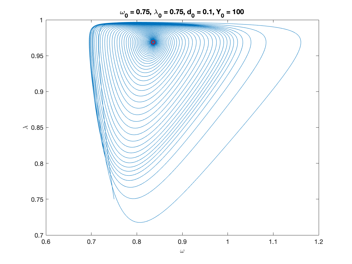
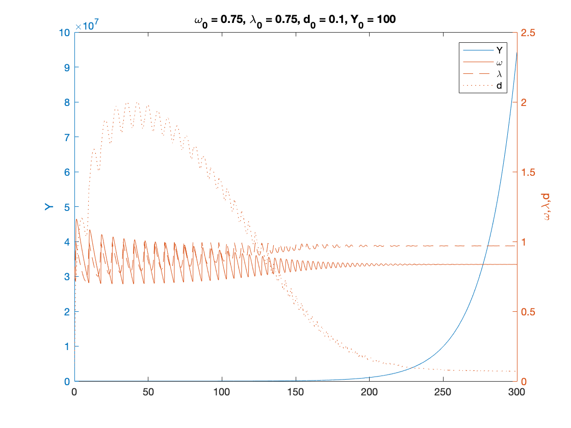
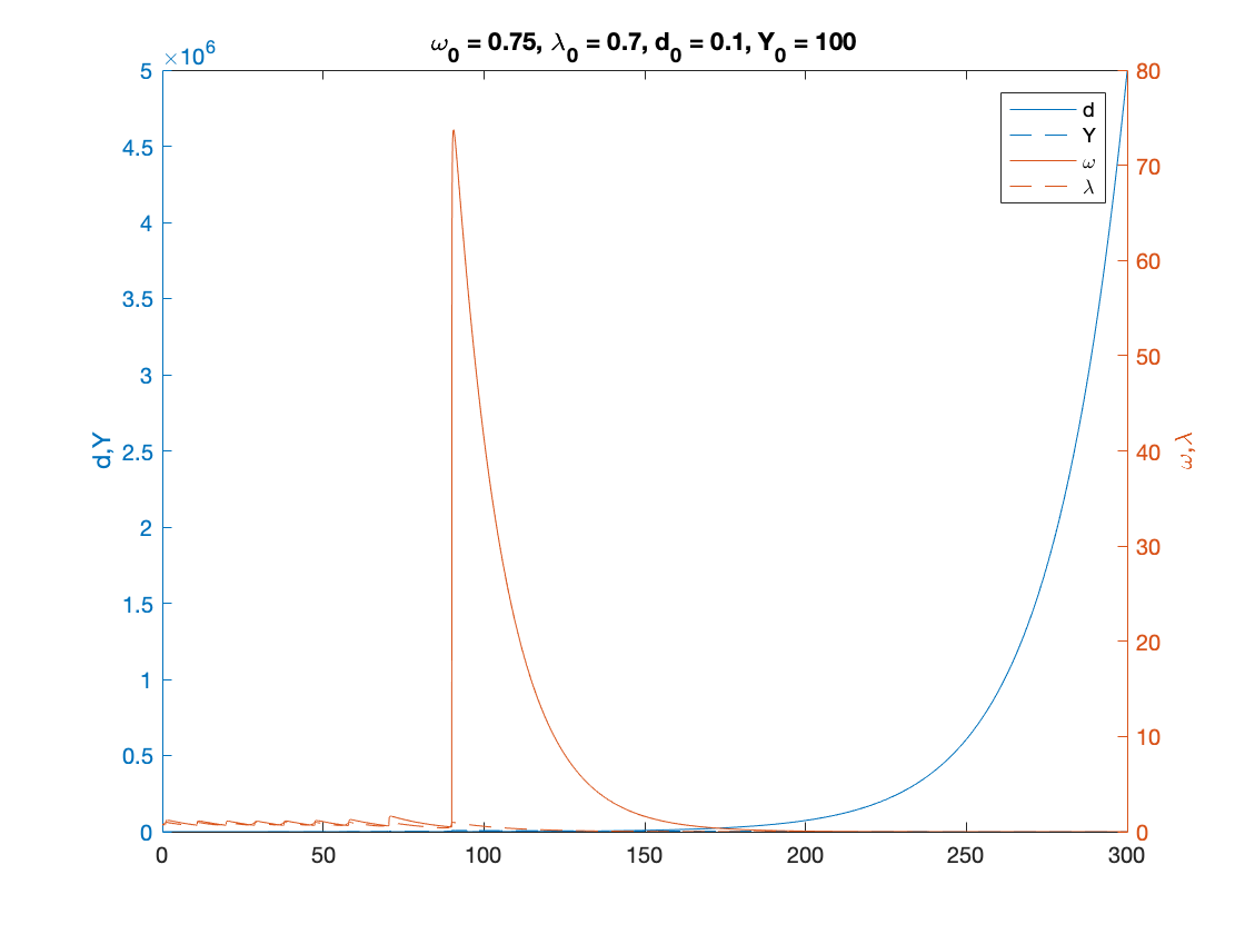
Sample paths of the Keen model
bar_pi_n_K = fun_kappa_inv(nu*(alpha+beta+delta));
bar_d_K = (fun_kappa(bar_pi_n_K)-bar_pi_n_K)/(alpha+beta);
bar_omega_K = 1-bar_pi_n_K-r*bar_d_K;
bar_lambda_K = fun_Phi_inv(alpha);

omega0 = 0.75;
lambda0 = 0.75;
d0 = 0.1;
Y0 = 100;
T = 300;

[tK,yK] = ode15s(@(t,y) keen(y), [0 T], convert([omega0, lambda0, d0]), options);
yK = retrieve(yK);
Y_output = Y0*yK(:,2)/lambda0.*exp((alpha+beta)*tK);

% Figure 3
figure(1)
plot(yK(:,1), yK(:,2)), hold on;
plot(bar_omega_K, bar_lambda_K, 'ro')
xlabel('\omega')
ylabel('\lambda')
title(['\omega_0 = ', num2str(omega0, txt_format), ...
    ', \lambda_0 = ', num2str(lambda0, txt_format), ...
    ', d_0 = ', num2str(d0, txt_format), ...
    ', Y_0 = ', num2str(Y0, txt_format)])
print('keen_phase_convergent','-depsc')


% Figure 4
figure(2)
yyaxis right
plot(tK, yK(:,1),tK,yK(:,2),tK,yK(:,3))
ylabel('\omega,\lambda,d')

yyaxis left
plot(tK, Y_output)
ylabel('Y')


title(['\omega_0 = ', num2str(omega0,txt_format), ...
    ', \lambda_0 = ', num2str(lambda0, txt_format), ...
    ', d_0 = ', num2str(d0, txt_format), ...
    ', Y_0 = ', num2str(Y0, txt_format)])
legend('Y','\omega', '\lambda','d')
print('keen_time_convergent','-depsc')


omega0 = 0.75;
lambda0 = 0.70;
d0 = 0.1;
Y0 = 100;
T = 300;

[tK,yK] = ode15s(@(t,y) keen(y), [0 T], convert([omega0, lambda0, d0]), options);
yK = retrieve(yK);
Y_output = Y0*yK(:,2)/lambda0.*exp((alpha+beta)*tK);

% Figure 5
figure(3)
yyaxis right
plot(tK, yK(:,1),tK,yK(:,2))
ylabel('\omega,\lambda')


yyaxis left
plot(tK,yK(:,3),tK, Y_output)
ylabel('d,Y')


title(['\omega_0 = ', num2str(omega0,txt_format), ...
    ', \lambda_0 = ', num2str(lambda0, txt_format), ...
    ', d_0 = ', num2str(d0, txt_format), ...
    ', Y_0 = ', num2str(Y0, txt_format)])
legend('d', 'Y','\omega','\lambda')
print('keen_time_divergent','-depsc')
Auxiliary functions
Instead of integrating the system in terms of omega, lambda and d, we decided to use:
log_omega = log(omega), tan_lambda = tan((lambda-0.5)*pi), and pi_n=1-omega-r*d log_p = log(p)
Experiments show that the numerical methods work better with these variables.
function new = convert(old)
    % This function converts
    % [omega, lambda, d, p]
    % to
    % [log_omega, tan_lambda, pi_n, log_p]
    % It also work with the first 2 or 3 elements alone.
    % each of these variables might also be a time-dependent vector

    n = size(old,2); %number of variables
    new = zeros(size(old));

    new(:,1) = log(old(:,1));
    new(:,2) = tan((old(:,2)-0.5)*pi);
    if n>2
        new(:,3) = 1-old(:,1)-r*old(:,3);
        if n==4
            new(:,4) = log(old(:,4));
        end
    end
end

function old = retrieve(new)
    % This function retrieves [omega, lambda, d, p]
    % from
    % [log_omega, tan_lambda, pi_n, log_p]
    %
    %  It also work with the first 2 or 3 elements alone.
    % each of these variables might also be a time-dependent vector

    n = size(new,2); %number of variables
    old = zeros(size(new));

    old(:,1) = exp(new(:,1));
    old(:,2) = atan(new(:,2))/pi+0.5;
    if n>2
        old(:,3) = (1-old(:,1)-new(:,3))/r;
        if n==4
            old(:,4) = exp(new(:,4));
        end
    end
end


function f = keen(y)
    f = zeros(3,1);
    log_omega = y(1);
    tan_lambda = y(2);
    pi_n = y(3);
    lambda = atan(tan_lambda)/pi+0.5;
    omega = exp(log_omega);
    g_Y = fun_kappa(pi_n)/nu-delta;

    % Equation (47)
    f(1) = fun_Phi(lambda)-alpha;                                   %d(log_omega)/dt
    f(2) = (1+tan_lambda^2)*pi*lambda*(g_Y-alpha-beta);             %d(tan_lambda)/dt
    f(3) = -omega*f(1)-r*(fun_kappa(pi_n)-pi_n)+(1-omega-pi_n)*g_Y; %d(pi_n)/dt
end
end