Contents
function out = keen_1995()
close all
clc
warning off
Parameters attribution and function definitions
par_alpha = 0.015;
par_beta = 0.035;
par_gamma = 0.02;
par_nu = 3;
par_A = 0.0000641;
par_D = 0.0400641;
fun_Phi = @(x) par_A./(1-x).^2- par_D;
fun_Phi_inv = @(y) 1 - sqrt(par_A./(y+par_D));
par_E = 0.0175 ;
par_F = 0.53;
par_G = 6;
par_H = 0.065;
fun_kappa = @(x) min(1,par_E./(par_F-(par_G/par_nu).*x).^2-par_H);
fun_kappa_inv = @(y) (par_nu/par_G)*(par_F-sqrt(par_E/(y+par_H)));
par_i = 0.05;
par_j = 1.2;
par_k = 4;
par_l = 0.05;
fun_Gamma = @(x) par_i./(par_j-par_k.*x).^2- par_l;
par_m = 0.0175;
par_n = 0.83;
par_o = 1.6014;
par_p = 0.039;
fun_Theta = @(x) par_m./(par_n-par_o.*x).^2- par_p;
TOL = 1E-7;
options = odeset('RelTol', TOL);
txt_format = '%3.3g';
Basic Goodwin limit cycle, page 617
figure(1)
tiledlayout(1,2)
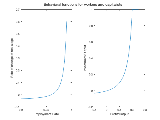
sgtitle('Behavioral functions for workers and capitalists')
nexttile
lambda_var=[0.9:0.001:0.99];
y1=fun_Phi(lambda_var);
plot(lambda_var,y1)
xlabel('Employment Rate')
ylabel('Rate of change of real wage')
nexttile
pi_var=[-0.1:0.001:0.25];
y2=fun_kappa(pi_var);
plot(pi_var,y2)
xlabel('Profit/Output')
ylabel('Investment/Output')
omega0 = 0.96;
lambda0 = 0.90;
T = 100;
lambda_bar = fun_Phi_inv(par_alpha);
omega_bar = 1-par_nu*(par_alpha+par_beta+par_gamma);
omega_mod = 1-fun_kappa_inv(par_nu*(par_alpha+par_beta+par_gamma));
par1 = [par_nu,par_alpha,par_beta,par_gamma,par_A,par_D];
par2 = [par_nu,par_alpha,par_beta,par_gamma,par_A,par_D,par_E,par_F,par_G,par_H];
[tG,yG] = ode15s(@(t,y) goodwin(y,par1), [0 T], [omega0, lambda0], options);
[tGmod,yGmod] = ode15s(@(t,y) goodwin_mod(y,par2), [0 T], [omega0, lambda0], options);
figure(2)
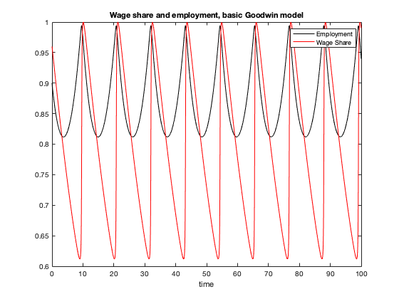
plot(tG, yG(:,2), 'k', tG, yG(:,1), 'r')
xlabel('time')
legend('Employment','Wage Share')
title(['Wage share and employment, basic Goodwin model'])
figure(3)
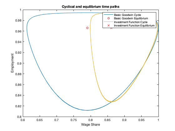
plot(yG(:,1), yG(:,2)), hold on;
plot(omega_bar, lambda_bar, 'ro')
plot(yGmod(:,1), yGmod(:,2))
plot(omega_mod, lambda_bar, 'rx')
legend('Basic Goodwin Cycle','Basic Goodwin Equilibrium','Investment Function Cycle',...
'Investment Function Equilibrium')
xlabel('Wage Share')
ylabel('Employment')
title(['Cyclical and equilibrium time paths'])
Base rate variations, page 620
par_xi = 0.036;
par_phi = 0;
kappa_eq = par_nu*(par_alpha+par_beta+par_gamma);
pi_eq=fun_kappa_inv(par_nu*(par_alpha+par_beta+par_gamma));
d_eq = (fun_kappa(pi_eq)-pi_eq-par_nu*par_gamma)/(par_alpha+par_beta-par_xi);
omega_eq = 1-pi_eq-par_xi*d_eq;
lambda_eq=fun_Phi_inv(par_alpha);
b_eq = par_xi*d_eq;
omega0 = 0.96;
lambda0 = 0.90;
d0 = 0.0;
y0 = [convert([omega0, lambda0]),d0];
T = 200;
par3 = [par_nu,par_alpha,par_beta,par_gamma,par_xi,par_phi,par_A,par_D,par_E,par_F,par_G,par_H];
[tK,yK] = ode15s(@(t,y) keen_wrong(y,par3), [0 T], y0, options);
yKnew = retrieve([yK(:,1),yK(:,2)]);
yK(:,1) = yKnew(:,1);
yK(:,2) = yKnew(:,2);
figure(4)
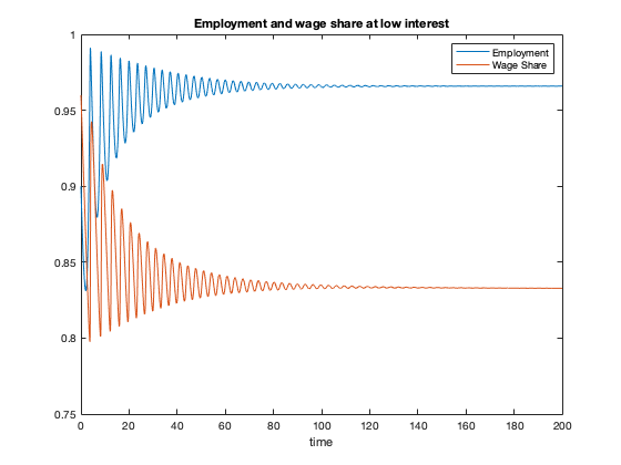
plot(tK, yK(:,2),tK,yK(:,1))
xlabel('time')
legend('Employment','Wage Share')
title(['Employment and wage share at low interest'])
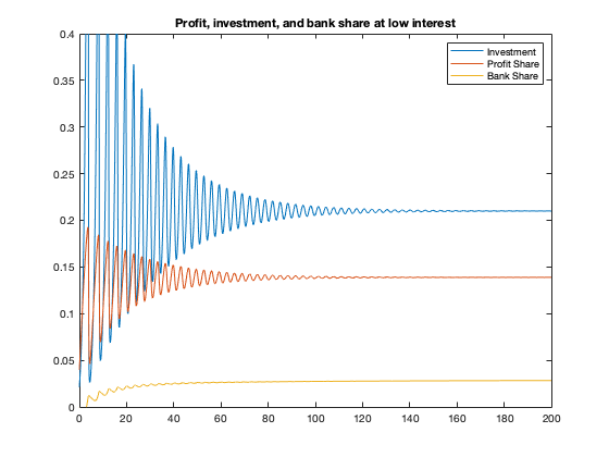
figure(5)
profit = 1-yK(:,1)-par_xi*yK(:,3);
invest = fun_kappa(profit);
bank = par_xi*yK(:,3);
plot(tK,invest,tK,profit,tK,bank)
legend('Investment','Profit Share','Bank Share')
ylim([0 0.4])
title(['Profit, investment, and bank share at low interest'])
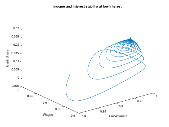
figure(6)
plot3(yK(:,2),yK(:,1),bank)
xlabel('Employment')
ylabel('Wages')
zlabel('Bank Share')
title(['Income and interest stability at low interest'])
par_xi = 0.04626;
par_phi = 0;
kappa_eq = par_nu*(par_alpha+par_beta+par_gamma);
pi_eq=fun_kappa_inv(par_nu*(par_alpha+par_beta+par_gamma));
d_eq = (fun_kappa(pi_eq)-pi_eq-par_nu*par_gamma)/(par_alpha+par_beta-par_xi);
omega_eq = 1-pi_eq-par_xi*d_eq;
lambda_eq=fun_Phi_inv(par_alpha);
b_eq = par_xi*d_eq;
omega0 = 0.96;
lambda0 = 0.90;
d0 = 0.0;
y0 = [convert([omega0, lambda0]),d0];
T = 1000;
par4 = [par_nu,par_alpha,par_beta,par_gamma,par_xi,par_phi,par_A,par_D,par_E,par_F,par_G,par_H];
[tK,yK] = ode15s(@(t,y) keen_wrong(y,par4), [0 T], y0, options);
yKnew = retrieve([yK(:,1),yK(:,2)]);
yK(:,1) = yKnew(:,1);
yK(:,2) = yKnew(:,2);
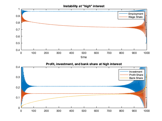
figure(7)
tiledlayout(2,1)
nexttile
plot(tK, yK(:,2),tK,yK(:,1))
xlabel('time')
legend('Employment','Wage Share')
title(['Instability at "high" interest'])
nexttile
profit = 1-yK(:,1)-par_xi*yK(:,3);
invest = fun_kappa(profit);
bank = par_xi*yK(:,3);
plot(tK,invest,tK,profit,tK,bank)
legend('Investment','Profit Share','Bank Share')
ylim([0 0.4])
title(['Profit, investment, and bank share at high interest'])
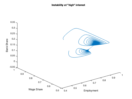
figure(8)
plot3(yK(:,2),yK(:,1),bank)
xlabel('Employment')
ylabel('Wage Share')
zlabel('Bank Share')
title(['Instability at "high" interest'])
Debt sensitivity variations, page 623
par_xi = 0.0459;
par_phi = 0.0022;
omega0 = 0.96;
lambda0 = 0.90;
d0 = 0.0;
y0 = [convert([omega0, lambda0]),d0];
T = 300;
par5 = [par_nu,par_alpha,par_beta,par_gamma,par_xi,par_phi,par_A,par_D,par_E,par_F,par_G,par_H];
[tK,yK] = ode15s(@(t,y) keen_wrong(y,par5), [0 T], y0, options);
yKnew = retrieve([yK(:,1),yK(:,2)]);
yK(:,1) = yKnew(:,1);
yK(:,2) = yKnew(:,2);
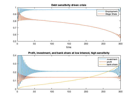
figure(9)
tiledlayout(2,1)
nexttile
plot(tK, yK(:,2),tK,yK(:,1))
xlabel('time')
legend('Employment','Wage Share')
title(['Debt sensitivity driven crisis'])
nexttile
profit = 1-yK(:,1)-(par_xi+par_phi*yK(:,3)).*yK(:,3);
invest = fun_kappa(profit);
bank = (par_xi+par_phi*yK(:,3)).*yK(:,3);
plot(tK,invest,tK,profit,tK,bank)
legend('investment','profit','bank share')
ylim([0 0.4])
title(['Profit, investment, and bank share at low interest, high sensitivity'])
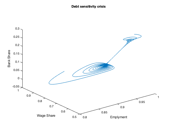
figure(10)
plot3(yK(:,2),yK(:,1),bank)
xlabel('Emplyment')
ylabel('Wage Share')
zlabel('Bank Share')
title(['Debt sensitivity crisis'])
Minskian government, page 625
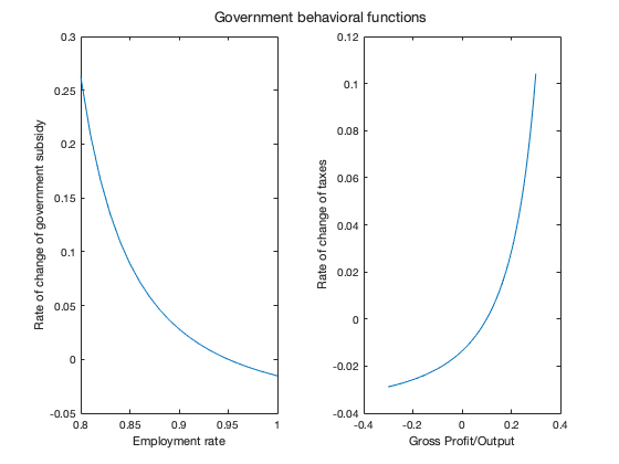
figure(11)
lambda_var = [0.8:0.01:1];
y3 = fun_Gamma(1-lambda_var);
pi_var = [-0.3:0.01:0.3];
y4 = fun_Theta(pi_var);
tiledlayout(1,2)
sgtitle('Government behavioral functions')
nexttile
plot(lambda_var,y3)
xlabel('Employment rate')
ylabel('Rate of change of government subsidy')
nexttile
plot(pi_var,y4)
xlabel('Gross Profit/Output')
ylabel('Rate of change of taxes')
omega0 = 0.96;
lambda0 = 0.90;
dk0 = 0;
dg0 = 0;
g0 = 0;
t0 = 0;
par_xi = 0.05;
par_phi = 0.005;
y0 = [convert([omega0, lambda0]),dk0,dg0,g0,t0];
T = 350;
par6 = [par_nu,par_alpha,par_beta,par_gamma,par_xi,par_phi,par_A,par_D,par_E,par_F,par_G,par_H,...
par_i,par_j,par_k,par_l,par_m,par_n,par_o,par_p];
[tG,yG] = ode15s(@(t,y) keen_government(y,par6), [0 T], y0, options);
yGnew = retrieve([yG(:,1),yG(:,2)]);
yG(:,1) = yGnew(:,1);
yG(:,2) = yGnew(:,2);
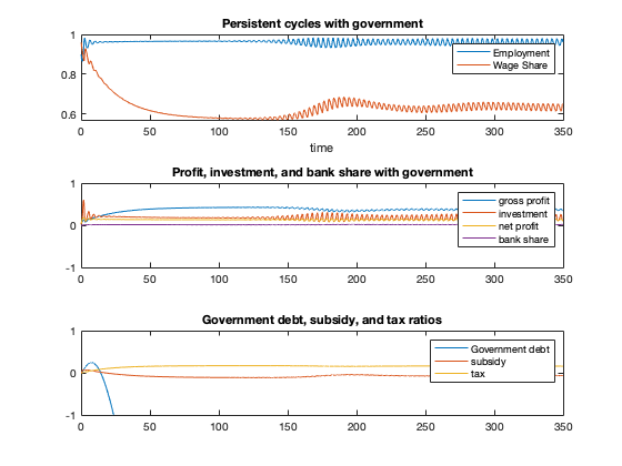
figure(12)
tiledlayout(3,1)
nexttile
plot(tG, yG(:,2),tG,yG(:,1))
xlabel('time')
legend('Employment','Wage Share')
title(['Persistent cycles with government'])
nexttile
profit = 1-yG(:,1)-(par_xi+par_phi*yG(:,3)).*yG(:,3)+yG(:,5)-yG(:,6);
gross_profit = 1-yG(:,1);
invest = fun_kappa(profit);
bank = (par_xi+par_phi*yG(:,3)).*yG(:,3);
plot(tG,gross_profit,tG,invest,tG,profit,tG,bank)
legend('gross profit','investment','net profit','bank share')
title(['Profit, investment, and bank share with government'])
ylim([-1,1])
nexttile
plot(tG, yG(:,4),tG,yG(:,5),tG,yG(:,6))
legend('Government debt','subsidy','tax')
title(['Government debt, subsidy, and tax ratios'])
ylim([-1,1])
figure(13)
tiledlayout(2,1)
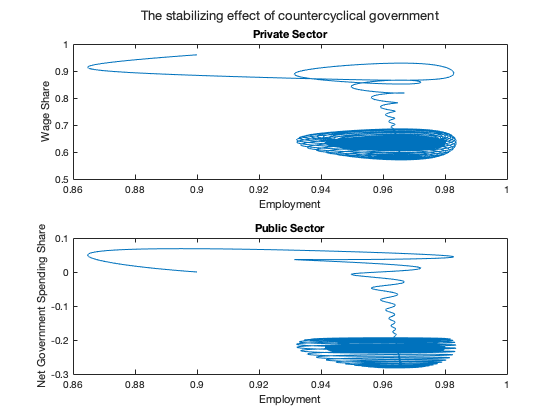
sgtitle(['The stabilizing effect of countercyclical government'])
nexttile
plot(yG(:,2), yG(:,1))
ylabel('Wage Share')
xlabel('Employment')
title(['Private Sector'])
nexttile
net_government = yG(:,5)-yG(:,6);
plot(yG(:,2), net_government)
ylabel('Net Government Spending Share')
xlabel('Employment')
title(['Public Sector'])
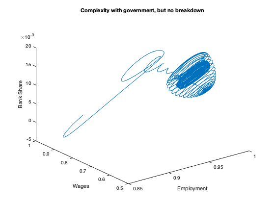
figure(14)
plot3(yG(:,2),yG(:,1),bank)
xlabel('Employment')
ylabel('Wages')
zlabel('Bank Share')
title(['Complexity with government, but no breakdown'])
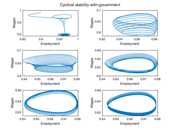
figure(15)
step=round(length(tG)/7);
tiledlayout(3,2)
sgtitle(['Cyclical stability with government'])
nexttile
plot(yG(1:2*step,2),yG(1:2*step,1))
xlabel('Employment')
ylabel('Wages')
nexttile
plot(yG(2*step:3*step,2),yG(2*step:3*step,1))
xlabel('Employment')
ylabel('Wages')
nexttile
plot(yG(3*step:4*step,2),yG(3*step:4*step,1))
xlabel('Employment')
ylabel('Wages')
nexttile
plot(yG(4*step:5*step,2),yG(4*step:5*step,1))
xlabel('Employment')
ylabel('Wages')
nexttile
plot(yG(5*step:6*step,2),yG(5*step:6*step,1))
xlabel('Employment')
ylabel('Wages')
nexttile
plot(yG(6*step:7*step,2),yG(6*step:7*step,1))
xlabel('Employment')
ylabel('Wages')


Auxiliary functions
function f = goodwin(y,par)
f = zeros(2,1);
omega = y(1);
lambda = y(2);
nu = par(1);
alpha = par(2);
beta = par(3);
gamma = par(4);
A = par(5);
D = par(6);
phillips = A./(1-lambda)^2- D;
f(1) = omega*(phillips-alpha);
f(2) = lambda*((1-omega)/nu-alpha-beta-gamma);
end
function f = goodwin_mod(y,par)
f = zeros(2,1);
omega = y(1);
lambda = y(2);
nu = par(1);
alpha = par(2);
beta = par(3);
gamma = par(4);
A = par(5);
D = par(6);
E = par(7);
F = par(8);
G = par(9);
H = par(10);
phillips = A./(1-lambda)^2- D;
kappa = E./(F-(G/nu).*(1-omega)).^2-H;
f(1) = omega*(phillips-alpha);
f(2) = lambda*(kappa/nu-alpha-beta-gamma);
end
function new = convert(old,r)
n = size(old,2);
new = zeros(size(old));
new(:,1) = log(old(:,1));
new(:,2) = tan((old(:,2)-0.5)*pi);
if n>2
new(:,3) = 1-old(:,1)-r*old(:,3);
if n==4
new(:,4) = log(old(:,4));
end
end
end
function old = retrieve(new,r)
n = size(new,2);
old = zeros(size(new));
old(:,1) = exp(new(:,1));
old(:,2) = atan(new(:,2))/pi+0.5;
if n>2
old(:,3) = (1-old(:,1)-new(:,3))/r;
if n==4
old(:,4) = exp(new(:,4));
end
end
end
function f = keen_wrong(y,par)
f = zeros(3,1);
log_omega = y(1);
tan_lambda = y(2);
d = y(3);
lambda = atan(tan_lambda)/pi+0.5;
omega = exp(log_omega);
nu = par(1);
alpha = par(2);
beta = par(3);
gamma = par(4);
xi = par(5);
phi = par(6);
A = par(7);
D = par(8);
E = par(9);
F = par(10);
G = par(11);
H = par(12);
r = xi+phi*d;
pi_n = 1-omega-r*d;
phillips = A./(1-lambda)^2- D;
kappa = E./(F-(G/nu).*pi_n).^2-H;
g_Y = kappa/nu-gamma;
f(1) = phillips-alpha;
f(2) = (1+tan_lambda^2)*pi*lambda*(g_Y-alpha-beta);
f(3) = r*d-pi_n+(nu-d)*(kappa/nu-gamma);
end
function f = keen_government(y,par)
f = zeros(6,1);
log_omega = y(1);
tan_lambda = y(2);
dk = y(3);
dg = y(4);
g = y(5);
t = y(6);
lambda = atan(tan_lambda)/pi+0.5;
omega = exp(log_omega);
nu = par(1);
alpha = par(2);
beta = par(3);
gamma = par(4);
xi = par(5);
phi = par(6);
A = par(7);
D = par(8);
E = par(9);
F = par(10);
G = par(11);
H = par(12);
i = par(13);
j = par(14);
k = par(15);
l = par(16);
m = par(17);
n = par(18);
o = par(19);
p = par(20);
r = xi+phi*(dk+dg);
pi_n = 1-omega-r.*dk+g-t;
phillips = A./(1-lambda)^2- D;
kappa = E./(F-(G/nu).*pi_n).^2-H;
Gamma = i./(j-k.*(1-lambda)).^2-l;
Theta = m./(n-o.*pi_n).^2-p;
g_Y = kappa/nu-gamma;
f(1) = phillips-alpha;
f(2) = (1+tan_lambda^2)*pi*lambda*(g_Y-alpha-beta);
f(3) = r*dk-(1-omega)+t-g+(nu-dk)*(kappa/nu-gamma);
f(4) = r*dg-dg*(kappa/nu-gamma)+g-t;
f(5) = Gamma - g*(kappa/nu-gamma);
f(6) = Theta - t*(kappa/nu-gamma);
end
end