Contents
- Base Parameters - Table 2
- Base initial conditions
- Other definitions
- Functions of interest
- Numerical Values of Interest
- Example 1 - fractional banking with finite equilibrium
- Example 2 - fractional banking with explosive equilibrium
- Example 3 - narrow banking with finite equilibirum
- Example 4 - narrow banking with explosive equilibirum
- Auxiliary functions
function out = narrow_paper()
%%%%%%%%%%%%%%%%%%%%%%%%%%%%%%%%%%%%%%%%%%%%%%%%%%%%%%%%%%%%%%%%%%%%%%%%%%%
% This code simulates the fractional and narrow banking models as
% specified in Grasselli and Lipton (2019)
%
% authors: M. Grasselli and A. Lipton
%%%%%%%%%%%%%%%%%%%%%%%%%%%%%%%%%%%%%%%%%%%%%%%%%%%%%%%%%%%%%%%%%%%%%%%%%%%
close all
clc
warning off
Base Parameters - Table 2
r = 0.03; %interest rate on loans NOTE: this is listed incorrectly as 0.04 in the paper
rd = 0.02;  %interest rate time deposits
rtheta = 0.012; % interest rate on bills
rm = 0.01; %interest rate on demand deposits

lambda10 = 0.3; % portfolio parameters for households
lambda20 = 0.3;
lambda30 = 0.3;
lambda11 = 4;
lambda12 = -1;
lambda22 = 2;

alpha = 0.025;       %productivity growth rate
beta = 0.02;         %population growth rate
eta_p = 0.35;        % adjustment speed for prices
markup = 1.65;       % mark-up value
gamma = 0.8;         % inflation sensitivity in the bargaining equation
g = 0.2;             % government spending
tax = 0.08;          % taxation
nu = 3;              %capital to output ratio
delta = 0.05;        %depreciation rate
kr = 0.08;           % capital adequacy ratio

phi0 = 0.0401;     %Phillips curve parameter
phi1 = 6.41e-05;   %Phillips curve parameter

kappa0 = -0.0065; %investment parameters
kappa1 = 0.8;
kappa2 = 1;
kappa3 = 1;     % NOTE: this is incorrectly listed in the paper as kappa3 = 2
kappa4 = 10;
xi = 4;

lambda00 = 1-(lambda10+lambda20+lambda30);  % proportion of households savings invested in cash
lambda1 = lambda10+lambda11*rtheta+lambda12*rm-(lambda11+lambda12)*rd; % proportion of households savings invested bills
lambda2 = lambda20+lambda12*rtheta+lambda22*rm-(lambda12+lambda22)*rd; % proportion of households savings invested demand deposits
lambda3 = lambda30-(lambda11+lambda12)*rtheta-(lambda12+lambda22)*rm+(lambda11+2*lambda12+lambda22)*rd; % proportion of households savings invested in time deposits
Base initial conditions
omega0  = 0.6;
lambda0 = 0.9;

Y0=100;

h0= 0.2;
thetah0 = 0.5;
mh0 = 0.2;

thetab0 = 0.1;
Other definitions
TOL = 1E-7;
options = odeset('RelTol', TOL);
txt_format = '%3.3g';
Functions of interest
inflation = @(x) eta_p*(markup*x-1);                                       % inflation, equation (2.64)

phillips = @(x) phi1./(1-x).^2- phi0;                                       % Phillips curve, equation (2.65)
phillips_prime = @(x) 2*phi1./(1-x).^3;                                     % derivative of phillips curve
phillips_inv = @(x) 1 - (phi1./(x+phi0)).^(1/2);                            % inverse of phillips curve

investment= @(x) kappa0+kappa1./(kappa2+kappa3.*exp(-kappa4*x)).^xi;        % investment function, equation (2.66)
% derivative of investment function
investment_prime= @(x) xi*kappa1*kappa3.*kappa4.*exp(-kappa4*x)./(kappa2+kappa3.*exp(-kappa4*x)).^(xi+1);
 % inverse of investment function
investment_inv = @(x) -log(((kappa1./(x-kappa0)).^(1/xi)-kappa2)/kappa3)/kappa4;
Numerical Values of Interest
pi_eq=investment_inv(nu*(alpha+beta+delta)) % profit share at interior equilibrium, equation (2.73)
pi_eq =

    0.1248
Example 1 - fractional banking with finite equilibrium
fR = 0.1; % reserve ratio

d0 = 0.4;
l0 = 0.6;
mf0 = ((1-kr)*l0+thetab0+(fR-1)*mh0-d0)/(1-fR);
cf0 = r*l0-rm*mf0;

T =100;

y0=[convert([omega0,lambda0]),l0,mf0,h0,thetah0,thetab0,mh0,d0];

[tK,yK] = ode15s(@(t,y) main(y), [0 T], y0, options);
sol = retrieve([yK(:,1),yK(:,2)]);

omega_sol=sol(:,1);
lambda_sol=sol(:,2);
l_sol=yK(:,3);
mf_sol=yK(:,4);

h_sol=yK(:,5);
theta_h_sol=yK(:,6);
theta_b_sol=yK(:,7);
mh_sol=yK(:,8);
d_sol=yK(:,9);

profit_sol = 1-tax-omega_sol-r*l_sol+rm*mf_sol;

Y_output = Y0*lambda_sol/lambda0.*exp((alpha+beta)*tK);

xb=l_sol+fR*(mh_sol+mf_sol)+theta_b_sol-(d_sol+mh_sol+mf_sol);
k_effective = xb./l_sol;

n=length(yK(:,1));

omega_bar = omega_sol(n);
lambda_bar = lambda_sol(n);
l_bar = l_sol(n);
mf_bar = mh_sol(n);
profit_bar = profit_sol(n);
investment_bar = investment(profit_bar);
growth_bar = investment_bar/nu -delta;
inflation_bar = inflation(omega_bar);

F1=phillips(lambda_bar)-(1-gamma)*inflation_bar-alpha;

F2=growth_bar-alpha-beta;

F3=-(growth_bar+inflation_bar)*l_bar+investment_bar+r*l_bar;

fprintf('\nExample 1 - fractional banking with finite equilibirum \n')
fprintf('omega = %f \n',omega_bar)
fprintf('e = %f \n',lambda_bar)
fprintf('l = %f \n',l_bar)
fprintf('mf = %f \n',mf_bar)
fprintf('profit = %f \n',profit_bar)
fprintf('investment = %f \n',investment_bar)
fprintf('growth = %f \n',growth_bar)
fprintf('inflation = %f \n',inflation_bar)

figure(1)
subplot(1,2,1)
plot(tK, omega_sol,tK,lambda_sol,tK,l_sol,tK,mf_sol)
xlabel('t')
ylabel('\omega,  e,  ell,  m_f')

yyaxis right
plot(tK, Y_output)
ylabel('Y')

title(['\omega_0 = ', num2str(omega0,txt_format), ...
    ', e_0 = ', num2str(lambda0, txt_format), ...
    ', l_0 = ', num2str(l0, txt_format),...
    ', m_{f0} = ', num2str(mf0,txt_format),...
    ', Y_0 = ', num2str(Y0, txt_format)])
legend('\omega', 'e',  'ell', 'm_f','Y')


%%%%%%%%%%%

subplot(1,2,2)
plot(tK,h_sol,tK,theta_h_sol,'--',tK,d_sol,'-.',tK,mh_sol,':',tK, theta_b_sol,':o','MarkerIndices',1:100:length(h_sol))
xlabel('t')
ylabel('h,  \theta_h,  d,  m_h, \theta_b')

title([' h_0 = ', num2str(h0, txt_format),...
    ', \theta_{h0} = ', num2str(thetah0, txt_format),...
    ', d_0 = ', num2str(d0, txt_format),...
    ', m_{h0} = ', num2str(mh0,txt_format),...
    ', \theta_{b0} = ', num2str(thetab0,txt_format)])
legend('h','\theta_h','d', 'm_h','\theta_b')

print('example1','-dpdf')
Example 1 - fractional banking with finite equilibirum
omega = 0.694728
e = 0.970586
l = 4.193678
mf = 0.757731
profit = 0.124946
investment = 0.285402
growth = 0.045134
inflation = 0.051205

Example 2 - fractional banking with explosive equilibrium
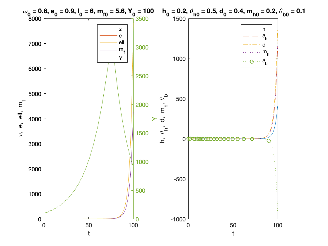
fR = 0.1; % reserve ratio

d0 = 0.4;
l0 = 6;
mf0 = ((1-kr)*l0+thetab0+(fR-1)*mh0-d0)/(1-fR);
cf0 = r*l0-rm*mf0;

T =100;

y0=[convert([omega0,lambda0]),l0,mf0,h0,thetah0,thetab0,mh0,d0];

[tK,yK] = ode15s(@(t,y) main(y), [0 T], y0, options);
sol = retrieve([yK(:,1),yK(:,2)]);

omega_sol=sol(:,1);
lambda_sol=sol(:,2);
l_sol=yK(:,3);
mf_sol=yK(:,4);

h_sol=yK(:,5);
theta_h_sol=yK(:,6);
theta_b_sol=yK(:,7);
mh_sol=yK(:,8);
d_sol=yK(:,9);

profit_sol = 1-tax-omega_sol-r*l_sol+rm*mf_sol;

Y_output = Y0*lambda_sol/lambda0.*exp((alpha+beta)*tK);

xb=l_sol+fR*(mh_sol+mf_sol)+theta_b_sol-(d_sol+mh_sol+mf_sol);
k_effective = xb./l_sol;

n=length(yK(:,1));

omega_bar = omega_sol(n);
lambda_bar = lambda_sol(n);
l_bar = l_sol(n);
mf_bar = mh_sol(n);
profit_bar = profit_sol(n);
investment_bar = investment(profit_bar);
growth_bar = investment_bar/nu -delta;
inflation_bar = inflation(omega_bar);

F1=phillips(lambda_bar)-(1-gamma)*inflation_bar-alpha;

F2=growth_bar-alpha-beta;

F3=-(growth_bar+inflation_bar)*l_bar+investment_bar+r*l_bar;

fprintf('\nExample 2 - fractional banking with explosive equilibirum \n')
fprintf('omega = %f \n',omega_bar)
fprintf('e = %f \n',lambda_bar)
fprintf('l = %f \n',l_bar)
fprintf('mf = %f \n',mf_bar)
fprintf('profit = %f \n',profit_bar)
fprintf('investment = %f \n',investment_bar)
fprintf('growth = %f \n',growth_bar)
fprintf('inflation = %f \n',inflation_bar)

figure(2)
subplot(1,2,1)
plot(tK, omega_sol,tK,lambda_sol,tK,l_sol,tK,mf_sol)
xlabel('t')
ylabel('\omega,  e,  ell,  m_f')

yyaxis right
plot(tK, Y_output)
ylabel('Y')

title(['\omega_0 = ', num2str(omega0,txt_format), ...
    ', e_0 = ', num2str(lambda0, txt_format), ...
    ', l_0 = ', num2str(l0, txt_format),...
    ', m_{f0} = ', num2str(mf0,txt_format),...
    ', Y_0 = ', num2str(Y0, txt_format)])
legend('\omega', 'e',  'ell', 'm_f','Y')


%%%%%%%%%%%

subplot(1,2,2)
plot(tK,h_sol,tK,theta_h_sol,'--',tK,d_sol,'-.',tK,mh_sol,':',tK, theta_b_sol,':o','MarkerIndices',1:100:length(h_sol))
xlabel('t')
ylabel('h,  \theta_h,  d,  m_h, \theta_b')

title([' h_0 = ', num2str(h0, txt_format),...
    ', \theta_{h0} = ', num2str(thetah0, txt_format),...
    ', d_0 = ', num2str(d0, txt_format),...
    ', m_{h0} = ', num2str(mh0,txt_format),...
    ', \theta_{b0} = ', num2str(thetab0,txt_format)])
legend('h','\theta_h','d', 'm_h','\theta_b')

print('example2','-dpdf')

%%%%%%%%%%%
Example 2 - fractional banking with explosive equilibirum
omega = 0.218466
e = 0.091358
l = 7819.682877
mf = 1184.538737
profit = -191.283881
investment = -0.006500
growth = -0.052167
inflation = -0.223836
Example 3 - narrow banking with finite equilibirum
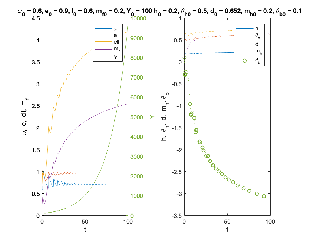
fR = 1; % reserve ratio

mf0 = 0.2;
l0 = 0.6;
d0 = (1-kr)*l0+thetab0;

cf0 = r*l0-rm*mf0;

T =100;

y0=[convert([omega0,lambda0]),l0,mf0,h0,thetah0,thetab0,mh0,d0];

[tK,yK] = ode15s(@(t,y) main(y), [0 T], y0, options);
sol = retrieve([yK(:,1),yK(:,2)]);

omega_sol=sol(:,1);
lambda_sol=sol(:,2);
l_sol=yK(:,3);
mf_sol=yK(:,4);

h_sol=yK(:,5);
theta_h_sol=yK(:,6);
theta_b_sol=yK(:,7);
mh_sol=yK(:,8);
d_sol=yK(:,9);

profit_sol = 1-tax-omega_sol-r*l_sol+rm*mf_sol;

Y_output = Y0*lambda_sol/lambda0.*exp((alpha+beta)*tK);

xb=l_sol+fR*(mh_sol+mf_sol)+theta_b_sol-(d_sol+mh_sol+mf_sol);
k_effective = xb./l_sol;

n=length(yK(:,1));

omega_bar = omega_sol(n);
lambda_bar = lambda_sol(n);
l_bar = l_sol(n);
mf_bar = mh_sol(n);
profit_bar = profit_sol(n);
investment_bar = investment(profit_bar);
growth_bar = investment_bar/nu -delta;
inflation_bar = inflation(omega_bar);

F1=phillips(lambda_bar)-(1-gamma)*inflation_bar-alpha;

F2=growth_bar-alpha-beta;

F3=-(growth_bar+inflation_bar)*l_bar+investment_bar+r*l_bar;

fprintf('\nExample 3 - narrow banking with finite equilibirum \n')
fprintf('omega = %f \n',omega_bar)
fprintf('e = %f \n',lambda_bar)
fprintf('l = %f \n',l_bar)
fprintf('mf = %f \n',mf_bar)
fprintf('profit = %f \n',profit_bar)
fprintf('investment = %f \n',investment_bar)
fprintf('growth = %f \n',growth_bar)
fprintf('inflation = %f \n',inflation_bar)

figure(3)
subplot(1,2,1)
plot(tK, omega_sol,tK,lambda_sol,tK,l_sol,tK,mf_sol)
xlabel('t')
ylabel('\omega,  e,  ell,  m_f')

yyaxis right
plot(tK, Y_output)
ylabel('Y')

title(['\omega_0 = ', num2str(omega0,txt_format), ...
    ', e_0 = ', num2str(lambda0, txt_format), ...
    ', l_0 = ', num2str(l0, txt_format),...
    ', m_{f0} = ', num2str(mf0,txt_format),...
    ', Y_0 = ', num2str(Y0, txt_format)])
legend('\omega', 'e',  'ell', 'm_f','Y')

%%%%%%%%%%%

subplot(1,2,2)
plot(tK,h_sol,tK,theta_h_sol,'--',tK,d_sol,'-.',tK,mh_sol,':',tK, theta_b_sol,':o','MarkerIndices',1:100:length(h_sol))
xlabel('t')
ylabel('h,  \theta_h,  d,  m_h, \theta_b')

title([' h_0 = ', num2str(h0, txt_format),...
    ', \theta_{h0} = ', num2str(thetah0, txt_format),...
    ', d_0 = ', num2str(d0, txt_format),...
    ', m_{h0} = ', num2str(mh0,txt_format),...
    ', \theta_{b0} = ', num2str(thetab0,txt_format)])
legend('h','\theta_h','d', 'm_h','\theta_b')

print('example3','-dpdf')
Example 3 - narrow banking with finite equilibirum
omega = 0.694781
e = 0.970579
l = 4.192916
mf = 0.646257
profit = 0.124910
investment = 0.285308
growth = 0.045103
inflation = 0.051236
Example 4 - narrow banking with explosive equilibirum
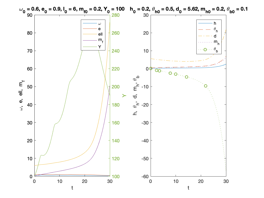
fR = 1; % reserve ratio

mf0 = 0.2;
l0 = 6;
d0 = (1-kr)*l0+thetab0;

cf0 = r*l0-rm*mf0;

T =30;

y0=[convert([omega0,lambda0]),l0,mf0,h0,thetah0,thetab0,mh0,d0];

[tK,yK] = ode15s(@(t,y) main(y), [0 T], y0, options);
sol = retrieve([yK(:,1),yK(:,2)]);

omega_sol=sol(:,1);
lambda_sol=sol(:,2);
l_sol=yK(:,3);
mf_sol=yK(:,4);

h_sol=yK(:,5);
theta_h_sol=yK(:,6);
theta_b_sol=yK(:,7);
mh_sol=yK(:,8);
d_sol=yK(:,9);

profit_sol = 1-tax-omega_sol-r*l_sol+rm*mf_sol;

Y_output = Y0*lambda_sol/lambda0.*exp((alpha+beta)*tK);

xb=l_sol+fR*(mh_sol+mf_sol)+theta_b_sol-(d_sol+mh_sol+mf_sol);
k_effective = xb./l_sol;

n=length(yK(:,1));

omega_bar = omega_sol(n);
lambda_bar = lambda_sol(n);
l_bar = l_sol(n);
mf_bar = mh_sol(n);
profit_bar = profit_sol(n);
investment_bar = investment(profit_bar);
growth_bar = investment_bar/nu -delta;
inflation_bar = inflation(omega_bar);

F1=phillips(lambda_bar)-(1-gamma)*inflation_bar-alpha;

F2=growth_bar-alpha-beta;

F3=-(growth_bar+inflation_bar)*l_bar+investment_bar+r*l_bar;

fprintf('\nExample 4 - narrow banking with explosive equilibirum \n')
fprintf('omega = %f \n',omega_bar)
fprintf('e = %f \n',lambda_bar)
fprintf('l = %f \n',l_bar)
fprintf('mf = %f \n',mf_bar)
fprintf('profit = %f \n',profit_bar)
fprintf('investment = %f \n',investment_bar)
fprintf('growth = %f \n',growth_bar)
fprintf('inflation = %f \n',inflation_bar)

figure(4)
subplot(1,2,1)
plot(tK, omega_sol,tK,lambda_sol,tK,l_sol,tK,mf_sol)
xlabel('t')
ylabel('\omega,  e,  ell,  m_f')

yyaxis right
plot(tK, Y_output)
ylabel('Y')

title(['\omega_0 = ', num2str(omega0,txt_format), ...
    ', e_0 = ', num2str(lambda0, txt_format), ...
    ', l_0 = ', num2str(l0, txt_format),...
    ', m_{f0} = ', num2str(mf0,txt_format),...
    ', Y_0 = ', num2str(Y0, txt_format)])
legend('\omega', 'e',  'ell', 'm_f','Y')


%%%%%%%%%%%

subplot(1,2,2)
plot(tK,h_sol,tK,theta_h_sol,'--',tK,d_sol,'-.',tK,mh_sol,':',tK, theta_b_sol,':o','MarkerIndices',1:100:length(h_sol))
xlabel('t')
ylabel('h,  \theta_h,  d,  m_h, \theta_b')

title([' h_0 = ', num2str(h0, txt_format),...
    ', \theta_{h0} = ', num2str(thetah0, txt_format),...
    ', d_0 = ', num2str(d0, txt_format),...
    ', m_{h0} = ', num2str(mh0,txt_format),...
    ', \theta_{b0} = ', num2str(thetab0,txt_format)])
legend('h','\theta_h','d', 'm_h','\theta_b')

print('example4','-dpdf')
Example 4 - narrow banking with explosive equilibirum
omega = 0.323247
e = 0.443312
l = 85.952861
mf = 6.240883
profit = -1.476233
investment = -0.006500
growth = -0.052167
inflation = -0.163325
Auxiliary functions
Instead of integrating the system in terms of omega, lambda and d, we decided to use:
log_omega = log(omega), tan_lambda = tan((lambda-0.5)*pi)
Experiments show that the numerical methods work better with these variables.
function new = convert(old)
    % This function converts
    % [omega, lambda]
    % to
    % [log_omega, tan_lambda]


    n = size(old,2); %number of variables
    new = zeros(size(old));

    new(:,1) = log(old(:,1));
    new(:,2) = tan((old(:,2)-0.5)*pi);
end

function old = retrieve(new)
    % This function retrieves [omega, lambda]
    % from
    % [log_omega, tan_lambda]

    n = size(new,2); %number of variables
    old = zeros(size(new));

    old(:,1) = exp(new(:,1));
    old(:,2) = atan(new(:,2))/pi+0.5;
end

function f = main(y)    % solves the main dynamical system
    f = zeros(9,1);

    log_omega = y(1);
    tan_lambda = y(2);
    l = y(3);
    mf= y(4);

    h=y(5);
    theta_h = y(6);
    theta_b = y(7);

    m_h = y(8);
    d = y(9);

    lambda = atan(tan_lambda)/pi+0.5;
    omega = exp(log_omega);
    profit = 1-tax-omega-r*l+rm*mf;

    growth = investment(profit)/nu-delta;    % real growth rate
    factor = g-tax-profit+rtheta*(theta_h+theta_b)+(1-kr)*investment(profit)-kr*r*l;

    % Equations (2.62), (2.67) and (2.70)-(2.72)
    f(1) = phillips(lambda)-(1-gamma)*inflation(omega)-alpha; %d(log_omega)/dt
    f(2) = (1+tan_lambda^2)*pi*lambda*(growth-alpha-beta); %d(tan_lambda)/dt
    f(3) = -(growth+inflation(omega))*l+investment(profit)+r*l; %d(l)/dt
    f(4) = -(growth+inflation(omega))*mf+profit+r*l;

    f(5) = -(growth+inflation(omega))*h+lambda00*factor; %dh/dt
    f(6) = -(growth+inflation(omega))*theta_h+lambda1*factor; %d(theta_h)/dt
    f(7) = -(growth+inflation(omega))*theta_b-(1-kr)*investment(profit)+(1-fR)*profit+(kr-fR)*r*l...
            +((1-fR)*lambda2+lambda3)*factor; %d(theta_b)/dt

    f(8) = -(growth+inflation(omega))*m_h+lambda2*factor; %d(m_h)/dt
    f(9) = -(growth+inflation(omega))*d+lambda3*factor; %d(d)/dt


end
end