Contents
function out = ponzi()
%%%%%%%%%%%%%%%%%%%%%%%%%%%%%%%%%%%%%%%%%%%%%%%%%%%%%%%%%%%%%%%%%%%%%%%%%%%
% This code simulates the Keen model with Ponzi financing
% as specified in Grasselli and Costa Lima (2012)
%
%
% authors: B. Costa Lima and M. Grasselli
%%%%%%%%%%%%%%%%%%%%%%%%%%%%%%%%%%%%%%%%%%%%%%%%%%%%%%%%%%%%%%%%%%%%%%%%%%%
close all
clc
warning off
Parameters attribution
Equations (24), (26), (63), (65) and (90)
nu = 3;              % capital-to-output ratio
alpha = 0.025;       % productivity growth rate
beta = 0.02;         % population growth rate
delta = 0.01;        % depreciation rate
phi0 = 0.04/(1-0.04^2); %Phillips curve parameter,  Phi(0.96)=0
phi1 = 0.04^3/(1-0.04^2); %Phillips curve parameter, Phi(0)=-0.04
r = 0.03;            %real interest rate
kappa0 = -0.0065 ;     % investment function parameter
kappa1 = exp(-5);      % investment function parameter
kappa2 = 20;           % investment function parameter
psi0 =-0.25;           % speculation function parameter
psi1 =0.25*exp(-0.36); % speculation function parameter
psi2 =12;
Other definitions
TOL = 1E-7;
options = odeset('RelTol', TOL);
txt_format = '%3.3g';
Functions Definition
fun_Phi = @(x) phi1./(1-x).^2- phi0;           % Phillips curve, equation (25)
fun_Phi_prime = @(x) 2*phi1./(1-x).^3;         % derivative of Phillips curve
fun_Phi_inv = @(x) 1 - (phi1/(x+phi0)).^(1/2); % inverse of Phillips curve

fun_kappa = @(x) kappa0+kappa1.*exp(kappa2.*x);         % Investment function, equation (64)
fun_kappa_prime = @(x) kappa1.*kappa2.*exp(kappa2.*x);  % Derivative of investment function
fun_kappa_inv = @(x) log((x-kappa0)./kappa1)./kappa2;   % Inverse of investment function

fun_Psi = @(x) psi0+psi1.*exp(psi2.*x);         % speculation function, equation (89)
Sample paths of the Keen model with speculation
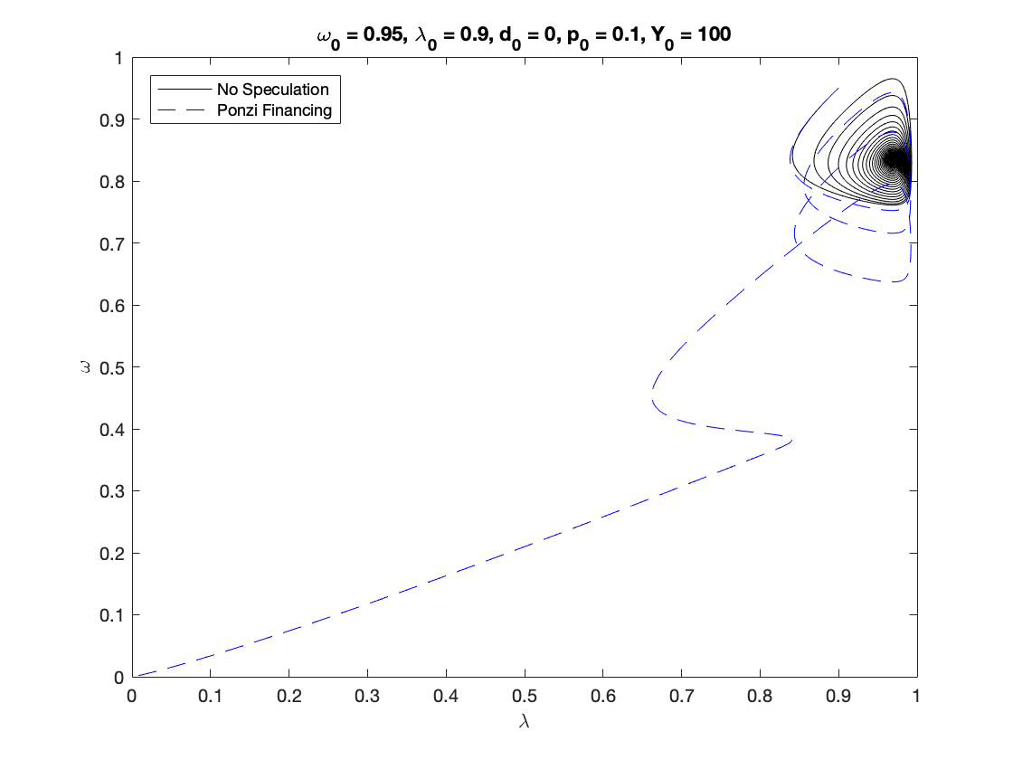
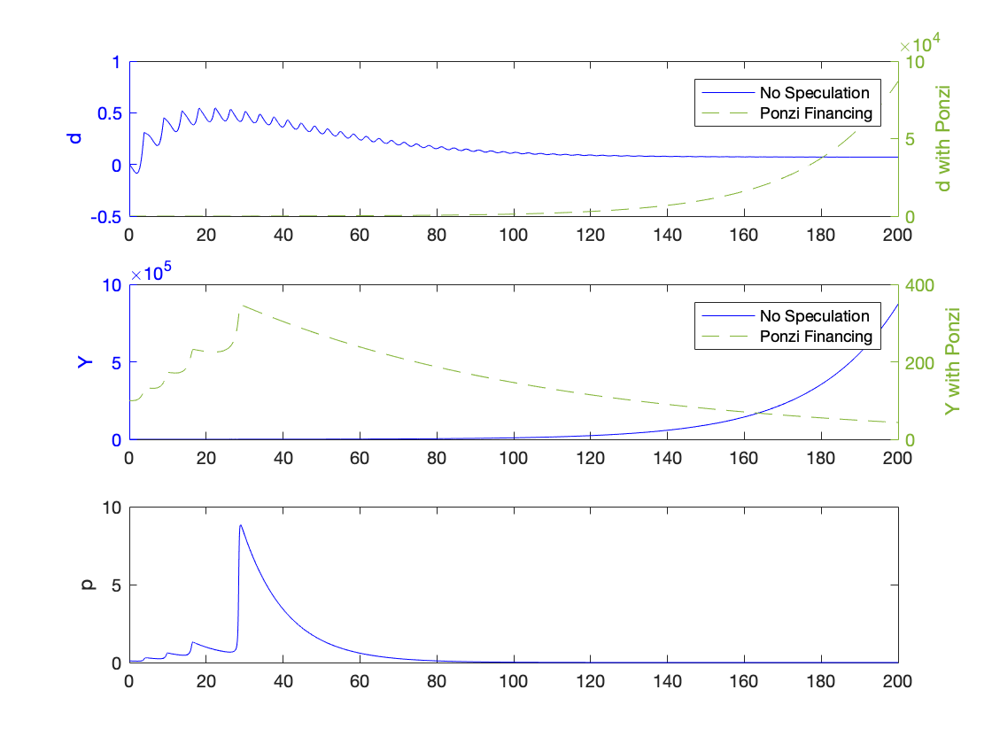
bar_pi_n_K = fun_kappa_inv(nu*(alpha+beta+delta));
bar_d_K = (fun_kappa(bar_pi_n_K)-bar_pi_n_K)/(alpha+beta);
bar_omega_K = 1-bar_pi_n_K-r*bar_d_K;
bar_lambda_K = fun_Phi_inv(alpha);

omega0 = 0.95;
lambda0 = 0.9;
d0 = 0;
p0 =0.1;
Y0 = 100;
T = 200;

[tK,yK] = ode15s(@(t,y) keen(y), [0 T], convert([omega0, lambda0, d0]), options);
yK = retrieve(yK);
Y_output = Y0*yK(:,2)/lambda0.*exp((alpha+beta)*tK);

[tP,yP] = ode15s(@(t,y) ponzi(y), [0 T], convert([omega0, lambda0, d0, p0]), options);
yP = retrieve(yP);
Y_output_ponzi = Y0*yP(:,2)/lambda0.*exp((alpha+beta)*tP);

% Figure 7
figure(1)
plot(yK(:,2), yK(:,1),'-k'), hold on;
plot(yP(:,2), yP(:,1),'--b')
xlabel('\lambda')
ylabel('\omega')
title(['\omega_0 = ', num2str(omega0, txt_format), ...
    ', \lambda_0 = ', num2str(lambda0, txt_format), ...
    ', d_0 = ', num2str(d0, txt_format), ...
    ', p_0 = ', num2str(p0, txt_format), ...
    ', Y_0 = ', num2str(Y0, txt_format)])
legend('No Speculation ', 'Ponzi Financing','Location','NorthWest')
print('keen_ponzi_phase','-depsc')

% Figure 8
figure(2)
fig = figure;
left_color = [0 0 1];
right_color = [0.5 0.7 0.2];
set(fig,'defaultAxesColorOrder',[left_color; right_color]);
title(['\omega_0 = ', num2str(omega0, txt_format), ...
    ', \lambda_0 = ', num2str(lambda0, txt_format), ...
    ', d_0 = ', num2str(d0, txt_format), ...
    ', p_0 = ', num2str(p0, txt_format), ...
    ', Y_0 = ', num2str(Y0, txt_format)])
subplot(3,1,1)
yyaxis right
plot(tP, yP(:,3),'--','color',[0.5 0.7 0.2]')
ylabel('d with Ponzi')

yyaxis left
plot(tK, yK(:,3),'-b')
ylabel('d')
legend('No Speculation ', 'Ponzi Financing','Location','NorthEast')

subplot(3,1,2)
yyaxis right
plot(tP, Y_output_ponzi,'--','color',[0.5 0.7 0.2]')
ylabel('Y with Ponzi')

yyaxis left
plot(tK, Y_output,'-b')
ylabel('Y')
legend('No Speculation ', 'Ponzi Financing','Location','NorthEast')

subplot(3,1,3)

plot(tP, yP(:,4),'-b')
ylabel('p')
print('keen_ponzi_time','-depsc')

Auxiliary functions
Instead of integrating the system in terms of omega, lambda and d, we decided to use:
log_omega = log(omega), tan_lambda = tan((lambda-0.5)*pi), and pi_n=1-omega-r*d log_p = log(p)
Experiments show that the numerical methods work better with these variables.
function new = convert(old)
    % This function converts
    % [omega, lambda, d, p]
    % to
    % [log_omega, tan_lambda, pi_n, log_p]
    % It also work with the first 2 or 3 elements alone.
    % each of these variables might also be a time-dependent vector

    n = size(old,2); %number of variables
    new = zeros(size(old));

    new(:,1) = log(old(:,1));
    new(:,2) = tan((old(:,2)-0.5)*pi);
    if n>2
        new(:,3) = 1-old(:,1)-r*old(:,3);
        if n==4
            new(:,4) = log(old(:,4));
        end
    end
end

function old = retrieve(new)
    % This function retrieves [omega, lambda, d, p]
    % from
    % [log_omega, tan_lambda, pi_n, log_p]
    %
    %  It also work with the first 2 or 3 elements alone.
    % each of these variables might also be a time-dependent vector

    n = size(new,2); %number of variables
    old = zeros(size(new));

    old(:,1) = exp(new(:,1));
    old(:,2) = atan(new(:,2))/pi+0.5;
    if n>2
        old(:,3) = (1-old(:,1)-new(:,3))/r;
        if n==4
            old(:,4) = exp(new(:,4));
        end
    end
end


function f = keen(y)
    f = zeros(3,1);
    log_omega = y(1);
    tan_lambda = y(2);
    pi_n = y(3);
    lambda = atan(tan_lambda)/pi+0.5;
    omega = exp(log_omega);
    g_Y = fun_kappa(pi_n)/nu-delta;

    % Equation (47)
    f(1) = fun_Phi(lambda)-alpha;                                   %d(log_omega)/dt
    f(2) = (1+tan_lambda^2)*pi*lambda*(g_Y-alpha-beta);             %d(tan_lambda)/dt
    f(3) = -omega*f(1)-r*(fun_kappa(pi_n)-pi_n)+(1-omega-pi_n)*g_Y; %d(pi_n)/dt
end

function f = ponzi(y)
    f = zeros(4,1);
    log_omega = y(1);
    tan_lambda = y(2);
    pi_n = y(3);
    log_p = y(4);
    lambda = atan(tan_lambda)/pi+0.5;
    omega = exp(log_omega);
    p = exp(log_p);
    g_Y = fun_kappa(pi_n)/nu-delta;

    % Equation (74)
    f(1) = fun_Phi(lambda)-alpha;                                       %d(log_omega)/dt
    f(2) = (1+tan_lambda^2)*pi*lambda*(g_Y-alpha-beta);                 %d(tan_lambda)/dt
    f(3) = -omega*f(1)-r*(fun_kappa(pi_n)-pi_n)+(1-omega-pi_n)*g_Y-r*p; %d(pi_n)/dt
    f(4) = fun_Psi(g_Y) - g_Y;                                          %dp/dt
end
end