Data are taken from Table 8.28 on page 326 of Rosner, Fundamentals of Biostatistics, Fifth edition.
The purpose of this study was to demonstrate that soy beans inoculated with nitrogen-fixing bacteria grow adequately without the use of expensive and environmentally deleterious synthesized fertilizers.
> podwt <- data.frame(wt=c(1.76,1.45,1.03,1.53,2.34,1.96,1.79,1.21,0.49,0.85,1,1.54,1.01,0.75,2.11,0.92),
treat=factor(c(rep("I",8),rep("U",8))))
> podwt
     wt treat
1  1.76     I
2  1.45     I
3  1.03     I
4  1.53     I
5  2.34     I
6  1.96     I
7  1.79     I
8  1.21     I
9  0.49     U
10 0.85     U
11 1.00     U
12 1.54     U
13 1.01     U
14 0.75     U
15 2.11     U
16 0.92     U
Compute mean, variance and standard deviation for the inoculated and uninoculated groups separately.
> sapply(split(podwt$wt,podwt$treat),mean)
      I       U
1.63375 1.08375
> sapply(split(podwt$wt,podwt$treat),var)
        I         U
0.1763125 0.2598839
> sqrt(sapply(split(podwt$wt,podwt$treat),var))
        I         U
0.4198958 0.5097881
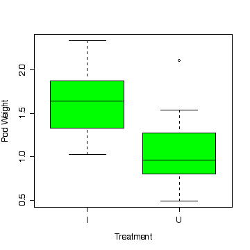
> boxplot(split(podwt$wt,podwt$treat),xlab="Treatment",ylab="Pod Weight",col="green")

Use lm() to fit a Linear Model, and store the result in the lm object fitpodwt.
> fitpodwt <- lm(wt~treat, data=podwt)
summary() displays the fitted coeficients and their t-tests.
> summary(fitpodwt)

Call:
lm(formula = wt ~ treat, data = podwt)

Residuals:
     Min       1Q   Median       3Q      Max
-0.60375 -0.25875 -0.09375  0.19875  1.02625

Coefficients:
            Estimate Std. Error t value Pr(>|t|)
(Intercept)   1.6338     0.1651   9.895 1.06e-07 ***
treatU       -0.5500     0.2335  -2.355   0.0336 *
---
Signif. codes:  0 `***' 0.001 `**' 0.01 `*' 0.05 `.' 0.1 ` ' 1

Residual standard error: 0.467 on 14 degrees of freedom
Multiple R-Squared: 0.2838,	Adjusted R-squared: 0.2327
F-statistic: 5.548 on 1 and 14 DF,  p-value: 0.03361
anova() displays the anova table.
> anova(fitpodwt)

Analysis of Variance Table

Response: wt
          Df Sum Sq Mean Sq F value  Pr(>F)
treat      1 1.2100  1.2100   5.548 0.03361 *
Residuals 14 3.0534  0.2181
---
Signif. codes:  0 `***' 0.001 `**' 0.01 `*' 0.05 `.' 0.1 ` ' 1
There is some evidence (P = 0.034) from these data that the treatment is effective.