These are model solutions. Students will get full marks if they do at least the graphs suggested, reach the main conclusions, and justify their conclusions graphically.
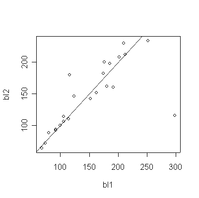
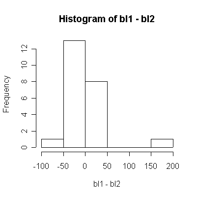
If it takes more than one day of fasting to reduce plasma carotene to suitable base levels, baseline 2 readings will be lower than baseline 1. The scatterplot shows excellent agreement between the two, with points more or less evenly scattered above and below the diagonal, except for subject #71 (in row 1) whose baseline 1 was much higher than baseline 2. The histogram shows that the difference between the two baseline measures is tightly scattered about 0, except for one outlier (subject #71). Hence I would use either baseline 2 or an average of the two, but not baseline 1.


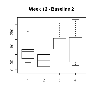
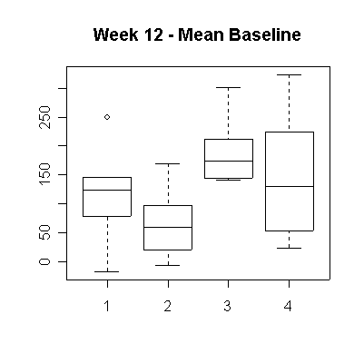
The following box plots of Week 12 minus baseline 1 and minus the mean baseline measure are almost the same. It is clear that Preparation 3 (BASF 30 mg) gives the greatest and most consistent elevation in plasma glucose levels. Preparation 4 (BASF 60 mg) is effective for some people, but overall is less consistent than Preparation 3. Preparation 2 (Roche 60 mg) is consistently the least effective.
 |
 |
There aren't many other graphs I could think of. This one shows the changes over 12 weeks relative to baseline 2 for each subject, with lines coded by preparation. It is not as simple to read as the boxplots. It shows that for most subjects, there was little change between weeks 6 and 12, suggesting that some treatments might achieve steady state levels of plasma carotene in less than 12 weeks.
The box plot of week 6 minus baseline 2 is similar to the boxplot for week 12 minus baseline 2, but the distribution for Preparation 3 is much more variable, suggesting that, for some subjects, Preparation 3 takes more than 6 weeks to achieve its final level.
> attach(betacar)
> windows(h=4,w=4)
> plot(bl1,bl2)
> abline(0,1)
> hist(bl1-bl2)
> boxplot(split(wk12-bl2,prep),main="Week 12 - Baseline 2")
> boxplot(split(wk12-(bl1+bl2)/2,prep),main="Week 12 - Mean Baseline")
> matplot(seq(6,12,by=2),rbind(wk6-bl2,wk8-bl2,wk10-bl2,wk12-bl2),type="l",col=prep,lty=prep,xlab="Week",ylab="Plasma Carotene")
> legend(7,350,paste("Prep",1:4),lty=1:4,col=1:4)
> title("Change from Baseline 2")
> boxplot(split(wk6-bl2,prep),main="Week 6 - Baseline 2")
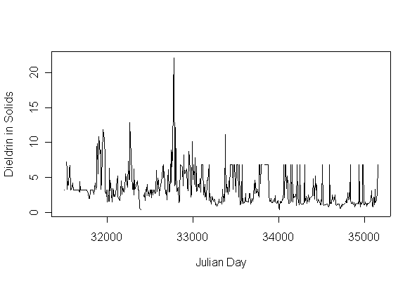
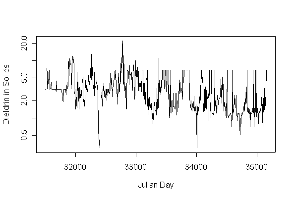
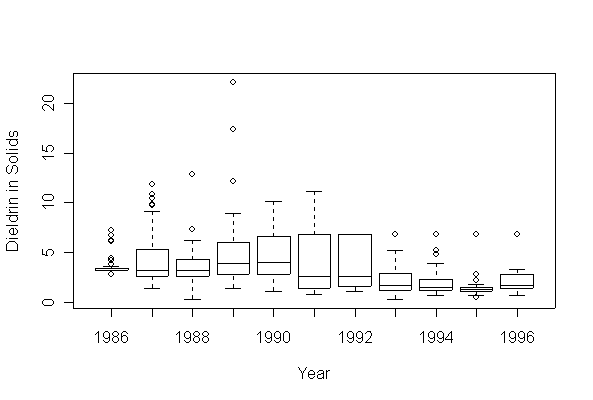
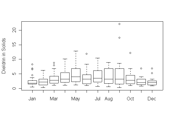
The time series plots show annual cycles throughout and a decreasing trend beginning in 1990. This is reinforced by the boxplots by year. The boxplots by month suggest that highest concentrations of dieldrin in solids are found in the summer months.
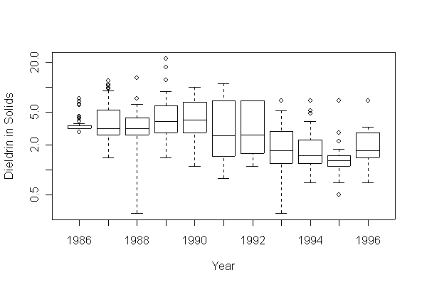
The decrease since 1990 shows mostly in a decreasing minimum value, and since this is a very low concentration, the downward trend is much more evident on a log scale. The log scale also makes the variation within months much more comparable, that is, the boxplots by month are more uniform in hinge spread on the log scale than in original units.
The detection limits were 3.2 ng/g up to 1989-02-09 and 6.8 ng/g from 1989-05-25. It is clear from the time series plot that the 6.8 ng/g is an upper detection limit, but the 3.2 ng/g could be either an upper limit or a lower limit as there are both higher and lower values recorded in the same time period.
While the upper detection limits prevent us from seeing if the extreme high values are decreasing after 1989, it is still evident that the bottom of the annual cycle is getting lower.
Because extreme high values occur only a few times in most years, replacement of extreme high values by upper detection limits will not affect the annual medians and lower quartiles in the box plots by year, provided that the upper detection limits are much higher than the annual medians. This is the case from May 1989 onward, where the upper detection limit is 6.8 ng/g.
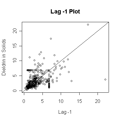
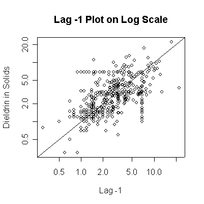
The Lag -1 plot shows moderate autocorrelation; on the log scale, the extreme high values have less impact and the scatter is more elliptical. The upper detection limits show as horizontal and vertical lines in the scatterplot.
 |
 |
> attach(diesol)
> windows(h=4,w=6)
> plot(julian,die.sol,type="l",xlab="Julian Day",ylab="Dieldrin in Solids")
> plot(julian,die.sol,type="l",xlab="Julian Day",ylab="Dieldrin in Solids",log="y")
> boxplot(split(die.sol,year),xlab="Year",ylab="Dieldrin in Solids")
> boxplot(split(die.sol,year),xlab="Year",ylab="Dieldrin in Solids",log="y")
> months <- c("Jan","Feb","Mar","Apr","May","Jun","Jul","Aug","Sep","Oct","Nov","Dec")
> boxplot(split(die.sol,month)[months],ylab="Dieldrin in Solids")
> boxplot(split(die.sol,month)[months],ylab="Dieldrin in Solids",log="y")
> windows(h=4,w=4)
> plot(die.sol[-length(die.sol)],die.sol[-1],xlab="Lag -1",ylab="Dieldrin in Solids",main="Lag -1 Plot")
> abline(0,1)
> plot(die.sol[-length(die.sol)],die.sol[-1],xlab="Lag -1",ylab="Dieldrin in Solids",main="Lag -1 Plot on Log Scale",log="xy")
> abline(0,1)
> diesol[dl,]
    julian year month day die.sol   dl
1    31504 1986   Apr   2     3.2 TRUE
2    31511 1986   Apr   9     3.2 TRUE
6    31539 1986   May   7     3.2 TRUE
11   31574 1986   Jun  11     3.2 TRUE
12   31588 1986   Jun  25     3.2 TRUE
15   31610 1986   Jul  17     3.2 TRUE
16   31617 1986   Jul  24     3.2 TRUE
17   31624 1986   Jul  31     3.2 TRUE
18   31631 1986   Aug   7     3.2 TRUE
19   31638 1986   Aug  14     3.2 TRUE
20   31645 1986   Aug  21     3.2 TRUE
21   31652 1986   Aug  28     3.2 TRUE
22   31659 1986   Sep   4     3.2 TRUE
23   31665 1986   Sep  10     3.2 TRUE
24   31673 1986   Sep  18     3.2 TRUE
27   31694 1986   Oct   9     3.2 TRUE
28   31701 1986   Oct  16     3.2 TRUE
29   31708 1986   Oct  23     3.2 TRUE
30   31715 1986   Oct  30     3.2 TRUE
31   31722 1986   Nov   6     3.2 TRUE
32   31730 1986   Nov  14     3.2 TRUE
33   31737 1986   Nov  21     3.2 TRUE
34   31743 1986   Nov  27     3.2 TRUE
35   31750 1986   Dec   4     3.2 TRUE
36   31757 1986   Dec  11     3.2 TRUE
37   31764 1986   Dec  18     3.2 TRUE
41   31806 1987   Jan  29     3.2 TRUE
42   31813 1987   Feb   5     3.2 TRUE
43   31820 1987   Feb  12     3.2 TRUE
44   31827 1987   Feb  19     3.2 TRUE
45   31834 1987   Feb  26     3.2 TRUE
46   31841 1987   Mar   5     3.2 TRUE
50   31870 1987   Apr   3     3.2 TRUE
59   31932 1987   Jun   4     3.2 TRUE
65   31981 1987   Jul  23     3.2 TRUE
67   31995 1987   Aug   6     3.2 TRUE
69   32009 1987   Aug  20     3.2 TRUE
79   32079 1987   Oct  29     3.2 TRUE
89   32191 1988   Feb  18     3.2 TRUE
99   32297 1988   Jun   3     3.2 TRUE
103  32324 1988   Jun  30     3.2 TRUE
105  32366 1988   Aug  11     3.2 TRUE
106  32373 1988   Aug  18     3.2 TRUE
123  32499 1988   Dec  22     3.2 TRUE
124  32507 1988   Dec  30     3.2 TRUE
126  32520 1989   Jan  12     3.2 TRUE
127  32527 1989   Jan  19     3.2 TRUE
129  32541 1989   Feb   2     3.2 TRUE
130  32548 1989   Feb   9     3.2 TRUE
141  32653 1989   May  25     6.8 TRUE
169  32856 1989   Dec  14     6.8 TRUE
173  32898 1990   Jan  25     6.8 TRUE
188  33010 1990   May  17     6.8 TRUE
201  33101 1990   Aug  16     6.8 TRUE
202  33108 1990   Aug  23     6.8 TRUE
203  33115 1990   Aug  30     6.8 TRUE
212  33185 1990   Nov   8     6.8 TRUE
244  33437 1991   Jul  18     6.8 TRUE
245  33444 1991   Jul  25     6.8 TRUE
246  33451 1991   Aug   1     6.8 TRUE
247  33458 1991   Aug   8     6.8 TRUE
249  33472 1991   Aug  22     6.8 TRUE
250  33479 1991   Aug  29     6.8 TRUE
251  33486 1991   Sep   5     6.8 TRUE
253  33507 1991   Sep  26     6.8 TRUE
254  33514 1991   Oct   3     6.8 TRUE
255  33521 1991   Oct  10     6.8 TRUE
256  33528 1991   Oct  17     6.8 TRUE
258  33542 1991   Oct  31     6.8 TRUE
262  33570 1991   Nov  28     6.8 TRUE
290  33773 1992   Jun  18     6.8 TRUE
291  33780 1992   Jun  25     6.8 TRUE
293  33794 1992   Jul   9     6.8 TRUE
294  33801 1992   Jul  16     6.8 TRUE
295  33808 1992   Jul  23     6.8 TRUE
297  33815 1992   Jul  30     6.8 TRUE
299  33829 1992   Aug  13     6.8 TRUE
301  33836 1992   Aug  20     6.8 TRUE
302  33843 1992   Aug  27     6.8 TRUE
303  33850 1992   Sep   3     6.8 TRUE
304  33857 1992   Sep  10     6.8 TRUE
305  33864 1992   Sep  17     6.8 TRUE
306  33871 1992   Sep  24     6.8 TRUE
307  33878 1992   Oct   1     6.8 TRUE
331  34060 1993   Apr   1     6.8 TRUE
333  34074 1993   Apr  15     6.8 TRUE
334  34081 1993   Apr  22     6.8 TRUE
342  34137 1993   Jun  17     6.8 TRUE
345  34158 1993   Jul   8     6.8 TRUE
353  34214 1993   Sep   2     6.8 TRUE
357  34242 1993   Sep  30     6.8 TRUE
365  34298 1993   Nov  25     6.8 TRUE
391  34509 1994   Jun  24     6.8 TRUE
402  34592 1994   Sep  15     6.8 TRUE
430  34830 1995   May  11     6.8 TRUE
445  34934 1995   Aug  23     6.8 TRUE
451  34977 1995   Oct   5     6.8 TRUE
452  34984 1995   Oct  12     6.8 TRUE
475  35152 1996   Mar  28     6.8 TRUE