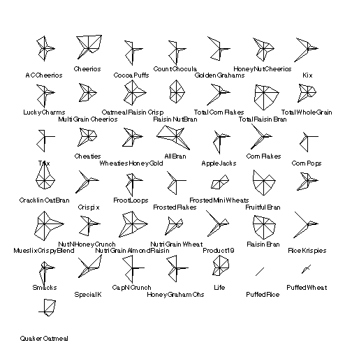
There are 8 variables and 43 observations. The stars plot facilitates cluster analysis (finding cereals that are similar to each other) but in all 8 dimensions.
> stars(cereal[,-1])

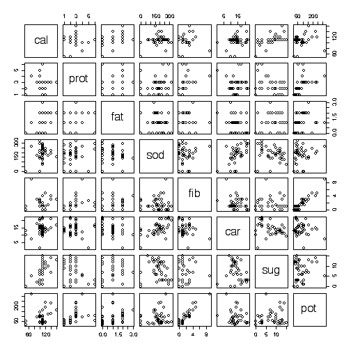
The pairs plot shows which pairs of variables are correlated.
> pairs(cereal[,-1])
Here is the PCA.
> pcacereal <- princomp(cereal[,-1], cor = T)
> pcacereal
Call:
princomp(x = cereal[, -1], cor = T)

Standard deviations:
   Comp.1    Comp.2    Comp.3    Comp.4    Comp.5    Comp.6    Comp.7
1.5961107 1.3618964 1.3299737 0.9318172 0.7051956 0.5978532 0.2459743
   Comp.8
0.2128916

 8  variables and  43 observations.
> summary(pcacereal)
Importance of components:
                          Comp.1    Comp.2    Comp.3    Comp.4    Comp.5
Standard deviation     1.5961107 1.3618964 1.3299737 0.9318172 0.7051956
Proportion of Variance 0.3184462 0.2318452 0.2211037 0.1085354 0.0621626
Cumulative Proportion  0.3184462 0.5502914 0.7713951 0.8799306 0.9420932
                           Comp.6      Comp.7      Comp.8
Standard deviation     0.59785320 0.245974321 0.212891551
Proportion of Variance 0.04467856 0.007562921 0.005665352
Cumulative Proportion  0.98677173 0.994334648 1.000000000
> pcacereal$load

Loadings:
     Comp.1 Comp.2 Comp.3 Comp.4 Comp.5 Comp.6 Comp.7 Comp.8
cal   0.114  0.657 -0.135  0.100  0.454  0.136  0.469  0.289
prot  0.421 -0.228 -0.253  0.372  0.551 -0.420 -0.242 -0.171
fat   0.316  0.302  0.166  0.687 -0.432  0.251 -0.125 -0.209
sod          0.273 -0.592        -0.502 -0.556
fib   0.558 -0.135        -0.376         0.194  0.453 -0.525
car  -0.238  0.113 -0.632         0.132  0.535 -0.370 -0.297
sug          0.566  0.362 -0.375  0.124 -0.254 -0.435 -0.371
pot   0.583               -0.296 -0.116  0.211 -0.409  0.585

               Comp.1 Comp.2 Comp.3 Comp.4 Comp.5 Comp.6 Comp.7 Comp.8
SS loadings     1.000  1.000  1.000  1.000  1.000  1.000  1.000  1.000
Proportion Var  0.125  0.125  0.125  0.125  0.125  0.125  0.125  0.125
Cumulative Var  0.125  0.250  0.375  0.500  0.625  0.750  0.875  1.000
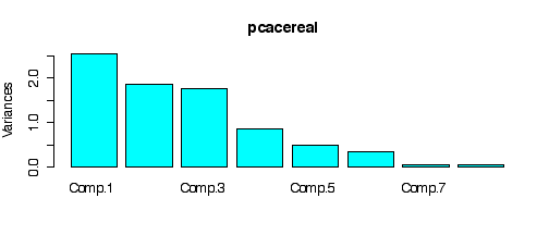
The screeplot from PCA indicates that the first three principal components might suffice.
> plot(pcacereal, col="cyan")
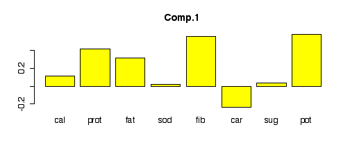
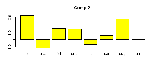
Here are the loadings of each component. Since fib
and pot had the strongest correlation of any pair in the
pairs plot, they show up with large, nearly equal weights in the
first component. Similarly, cal and sug are
also correlated and show up with large, nearly equal weights in the
second component. Subsequent components become harder to interpret.
> barplot(pcacereal$load[,1], col="yellow", main="Comp.1")
> barplot(pcacereal$load[,2], col="yellow", main="Comp.2")
> barplot(pcacereal$load[,3], col="yellow", main="Comp.3")
> barplot(pcacereal$load[,4], col="yellow", main="Comp.4")
> barplot(pcacereal$load[,5], col="yellow", main="Comp.5")
> barplot(pcacereal$load[,6], col="yellow", main="Comp.6")
> barplot(pcacereal$load[,7], col="yellow", main="Comp.7")
> barplot(pcacereal$load[,8], col="yellow", main="Comp.8")
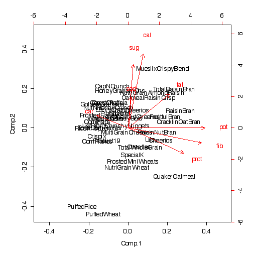
The biplot computes the score for each cereal from the loadings in Component 1 and Component 2, and plots one component against the other. The red arrows show the directions of the original axes in the Comp.1 x Comp.2 space. Note how related cereals are placed near each other on this plot; visual cluster analysis has been made possible in just 2 dimensions.
> biplot(pcacereal)
The following printouts confirm that PCA is just an eigenanalysis of the correlation matrix. The signs of the loadings are all reversed from the matrix of eigenvectors, but that doesn't matter, it is the same solution.
> eigen(cor(cereal[,-1]))
$values
[1] 2.54756944 1.85476179 1.76882996 0.86828336 0.49730081 0.35742845
[7] 0.06050337 0.04532281

$vectors
            [,1]          [,2]        [,3]        [,4]        [,5]
[1,] -0.11428766 -0.6565978346  0.13512273  0.10047942  0.45370278
[2,] -0.42083604  0.2279411416  0.25306331  0.37167686  0.55136283
[3,] -0.31568965 -0.3017868744 -0.16564583  0.68746001 -0.43196553
[4,] -0.02253715 -0.2730761901  0.59171072 -0.07540825 -0.50184839
[5,] -0.55812331  0.1346700401  0.06964853 -0.37635107 -0.07569865
[6,]  0.23809310 -0.1134578294  0.63159218 -0.05877830  0.13150590
[7,] -0.03833510 -0.5659218032 -0.36206814 -0.37491534  0.12379085
[8,] -0.58310200  0.0001015048  0.07271691 -0.29633765 -0.11557910
           [,6]        [,7]        [,8]
[1,]  0.1357808  0.46893535  0.28858336
[2,] -0.4203738 -0.24231470 -0.17124143
[3,]  0.2513099 -0.12505885 -0.20936646
[4,] -0.5557961  0.08693274  0.02819652
[5,]  0.1942594  0.45295861 -0.52462634
[6,]  0.5348405 -0.36979311 -0.29661480
[7,] -0.2536404 -0.43507631 -0.37102432
[8,]  0.2113266 -0.40862740  0.58471744

> sqrt(eigen(cor(cereal[,-1]))$val)
[1] 1.5961107 1.3618964 1.3299737 0.9318172 0.7051956 0.5978532 0.2459743
[8] 0.2128916