The function skew(x) computes the skewness coefficient g1 for an array of observations x.
> skew
function(x)
{
        mean((x - mean(x))^3)/((mean((x - mean(x))^2))^1.5)
}
The function excess(x) computes the coefficient of excess g2 for an array of observations x.
> excess
function(x)
{
        (mean((x - mean(x))^4)/((mean((x - mean(x))^2))^2)) - 3
}
The function normex(n, nboot, theta) generates nboot independent random samples, each with n observations, from a standard normal distribution, and places them in a matrix. A user-specified function theta() is applied to each row of the matrix, returning a vector of theta() values for the nboot samples.
> normex
function(n, nboot, theta)
{
        data <- matrix(rnorm(n * nboot), nrow = nboot)
        apply(data, 1, theta)
}
The function gammex(n, nboot, theta, al) generates nboot independent random samples, each with n observations, from a gamma distribution with shape parameter al, and places them in a matrix. A user-specified function theta() is applied to each row of the matrix, returning a vector of theta() values for the nboot samples.
> gammex
function(n, nboot, theta, al)
{
        data <- matrix(rgamma(n * nboot, al), nrow = nboot)
        apply(data, 1, theta)
}
These functions can be used to study the sampling distributions of g1 and g2 for different sample sizes n and, in the case of the gamma distribution, for different values of the shape parameter al. A histogram is a useful way to display the results. Pick nboot large enough to give a smooth histogram but not so large that the computation takes too long.
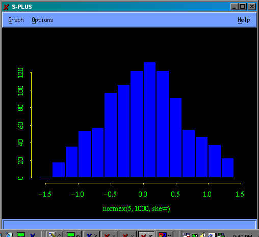
> hist(normex(5,1000,skew))
The simulated values of g1 are distributed more or less symmetrically about the true value, which is 0.
> hist(normex(5,1000,excess))
Most of the simulated values of g2 are much less than the true value, which is 0.
> hist(gammex(5,1000,skew,1.5))
All of the simulated values of g1 are less than the true value, which is 2 / sqrt(1.5) = 1.63.
> hist(gammex(5,1000,excess,1.5))
All of the simulated values of g2 are much less than the true value, which is 6 / 1.5 = 4.