Lab 2: solutions
© 2005 Ben Bolker
Exercise 1: nothing to do
Exercise 2:
Re-create the data frame to play with:
> loc = factor(rep(LETTERS[1:3], 2))
> day = factor(rep(1:2, each = 3))
> set.seed(1001)
> val = round(runif(6), 3)
> d = data.frame(loc, day, val)
> d
  loc day   val
1   A   1 0.986
2   B   1 0.413
3   C   1 0.430
4   A   2 0.419
5   B   2 0.427
6   C   2 0.888
Separate data with one row for each
location and one column for each day:
> unstack(d, val ~ day)
     X1    X2
1 0.986 0.419
2 0.413 0.427
3 0.430 0.888
Because R doesn't allow numbers
alone as column names, it puts
an X in front of the values
of day to get the column
names X1 and X2.
Separate data with one row for each
day and one column for each location:
> unstack(d, val ~ loc)
      A     B     C
1 0.986 0.413 0.430
2 0.419 0.427 0.888
While less complicated than reshape(),
stack() and unstack() don't
preserve information very well: for example,
the row names in the first example are
not set to A, B, C.
Exercise 3:
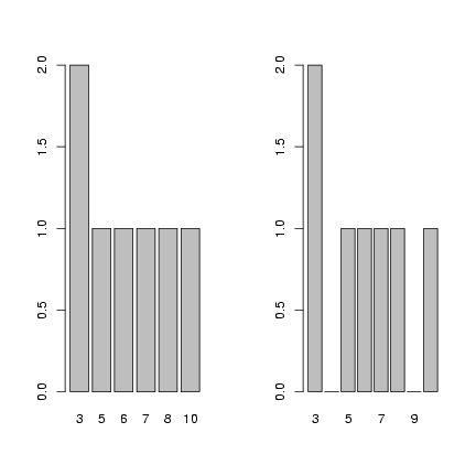
Use levels=3:10 to make sure that all values
between 3 and 10, even those not represented in
the data set, are included in the factor definition
and thus appear as zeros rather than being skipped
when you plot the factor.
> f = factor(c(3, 3, 5, 6, 7, 8, 10))
> op = par(mfrow = c(1, 2))
> plot(f)
> f = factor(c(3, 3, 5, 6, 7, 8, 10), levels = 3:10)
> plot(f)
> par(op)
 Exercise 4:
Read in and recreate the seed predation data
and table:
Exercise 4:
Read in and recreate the seed predation data
and table:
> data = read.table("seedpred.dat", header = TRUE)
> data$available = data$remaining + data$taken
> t1 = table(data$available, data$taken)
> v = as.numeric(log10(1 + t1))
> r = row(t1)
> c = col(t1)
Create versions of the variables that are
sorted in order of increasing values
of v (v_sorted=sort(v) would
have the same effect as the first line):
> v_sorted = v[order(v)]
> r_sorted = r[order(v)]
> c_sorted = c[order(v)]
Draw the plots:
> op = par(mfrow = c(2, 2), mgp = c(2, 1, 0), mar = c(4.2, 3, 1,
+     1))
> plot(sort(v))
> plot(v, col = r, pch = c)
> plot(v_sorted, col = r_sorted, pch = c_sorted)
> legend(0, 2.8, pch = 1, col = 1:5, legend = 1:5)
> legend(6, 2.8, pch = 1:6, col = 1, legend = 0:5)
> text(0, 3, "available", adj = 0)
> text(8, 3, "taken", adj = 0)
> par(op)
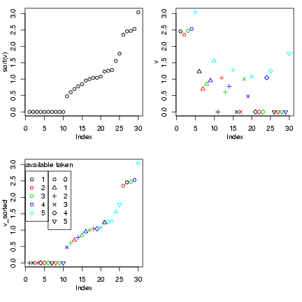 The first plot shows the sorted data;
the second plot shows the data coded
by color, and the third shows the
data sorted and coded (thanks to Ian
and Jeff for the idea of the legends).
I tweaked the margins and label spacing
slightly with mgp and mar
in the par() command.
In fact, this plot probably doesn't
give a lot of insights that aren't better
conveyed by the barplots or the bubble plot ...
Exercise 5:
Read in the data (again), take the
subset with 5 seeds available,
and generate the table
of (number taken) × (Species):
The first plot shows the sorted data;
the second plot shows the data coded
by color, and the third shows the
data sorted and coded (thanks to Ian
and Jeff for the idea of the legends).
I tweaked the margins and label spacing
slightly with mgp and mar
in the par() command.
In fact, this plot probably doesn't
give a lot of insights that aren't better
conveyed by the barplots or the bubble plot ...
Exercise 5:
Read in the data (again), take the
subset with 5 seeds available,
and generate the table
of (number taken) × (Species):
> data = read.table("seedpred.dat", header = TRUE)
> data2 = data
> data2$available = data2$remaining + data2$taken
> data2 = data2[data2$available == 5, ]
> t1 = table(data2$taken, data2$Species)
Draw the plots:
> op = par(mfrow = c(2, 1), mgp = c(2.5, 1, 0), mar = c(4.1, 3.5,
+     1.1, 1.1))
> logt1 = log10(1 + t1)
> barplot(logt1, beside = TRUE, ylab = "log10(1+taken)")
> library(gplots)
Loading required package: gdata
Loading required package: gtools

Attaching package: 'gplots'


	The following object(s) are masked from package:stats :

	 lowess
> barplot2(t1 + 1, beside = TRUE, log = "y", ylab = "taken+1")
> par(op)
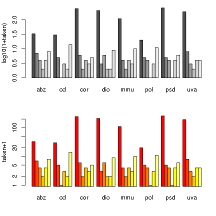 Once again, I'm using par() to tweak graphics
options and squeeze the plots a little closer together.
barplot2() has a log option that
lets us plot the values on a logarithmic scale
rather than converting to logs - but it hiccups
if we have 0 values, so we still have to plot
t1+1. (barplot2() also uses
different default bar colors.)
Exercise 6:
Read in the measles data again:
Once again, I'm using par() to tweak graphics
options and squeeze the plots a little closer together.
barplot2() has a log option that
lets us plot the values on a logarithmic scale
rather than converting to logs - but it hiccups
if we have 0 values, so we still have to plot
t1+1. (barplot2() also uses
different default bar colors.)
Exercise 6:
Read in the measles data again:
> data = read.table("ewcitmeas.dat", header = TRUE, na.strings = "*")
Separate out the
incidence data (columns 4 through 10), find
the minima and maxima by column, and compute the
range:
> incidence = data[, 4:10]
> imin = apply(incidence, 2, min, na.rm = TRUE)
> imax = apply(incidence, 2, max, na.rm = TRUE)
> irange = imax - imin
Another way to get the range: apply the
range() command, which will return
a matrix where the first row is the minima
and the second row - then subtract:
> iranges = apply(incidence, 2, range, na.rm = TRUE)
> iranges
     London Bristol Liverpool Manchester Newcastle Birmingham Sheffield
[1,]      1       0         0          0         0          0         0
[2,]   5464     835       813        894       616       2336       804
> irange = iranges[2, ] - iranges[1, ]
Or you could define a function that computes the difference:
> rangediff = function(x) {
+     diff(range(x, na.rm = TRUE))
+ }
> irange = apply(incidence, 2, rangediff)
Now use scale() to subtract the minimum and
divide by the range:
> scaled_incidence = scale(incidence, center = imin, scale = irange)
Checking:
> summary(scaled_incidence)
     London           Bristol          Liverpool         Manchester
 Min.   :0.00000   Min.   :0.00000   Min.   :0.00000   Min.   :0.00000
 1st Qu.:0.01501   1st Qu.:0.00479   1st Qu.:0.01968   1st Qu.:0.01119
 Median :0.03496   Median :0.01557   Median :0.05904   Median :0.03244
 Mean   :0.07665   Mean   :0.05710   Mean   :0.11312   Mean   :0.08352
 3rd Qu.:0.08915   3rd Qu.:0.04551   3rd Qu.:0.16697   3rd Qu.:0.09172
 Max.   :1.00000   Max.   :1.00000   Max.   :1.00000   Max.   :1.00000
 NA's   :1.00000   NA's   :1.00000   NA's   :2.00000
   Newcastle         Birmingham         Sheffield
 Min.   :0.00000   Min.   :0.000000   Min.   :0.000000
 1st Qu.:0.00487   1st Qu.:0.006849   1st Qu.:0.007463
 Median :0.01299   Median :0.020120   Median :0.023632
 Mean   :0.05199   Mean   :0.054013   Mean   :0.078439
 3rd Qu.:0.04383   3rd Qu.:0.048587   3rd Qu.:0.085821
 Max.   :1.00000   Max.   :1.000000   Max.   :1.000000
                   NA's   :1.000000
> apply(scaled_incidence, 2, range, na.rm = TRUE)
     London Bristol Liverpool Manchester Newcastle Birmingham Sheffield
[1,]      0       0         0          0         0          0         0
[2,]      1       1         1          1         1          1         1
Exercise 7:
You first need to calculate the column means
so you can tell sweep() to subtract them
(which is what scale(x,center=TRUE,scale=FALSE)
does):
> imean = colMeans(incidence, na.rm = TRUE)
> scaled_incidence = sweep(incidence, 2, imean, "-")
Check:
> c1 = colMeans(scaled_incidence, na.rm = TRUE)
> c1
       London       Bristol     Liverpool    Manchester     Newcastle
 4.789583e-12 -1.342629e-14  9.693277e-13 -9.520250e-13 -3.216842e-13
   Birmingham     Sheffield
 1.045927e-12 -2.389592e-13
(these numbers are very close to zero ... but not exactly equal,
because of round-off error)
> all(abs(c1) < 1e-11)
[1] TRUE
Exercise 8*:
Resurrect long-format data:
> date = as.Date(paste(data$year + 1900, data$mon, data$day, sep = "/"))
> city_names = colnames(data)[4:10]
> data = cbind(data, date)
> data_long = reshape(data, direction = "long", varying = list(city_names),
+     v.name = "incidence", drop = c("day", "mon", "year"), times = factor(city_names),
+     timevar = "city")
Calculate min, max, and range difference:
> city_max = tapply(data_long$incidence, data_long$city, max, na.rm = TRUE)
> city_min = tapply(data_long$incidence, data_long$city, min, na.rm = TRUE)
> range1 = city_max - city_min
> scdat1 = data_long$incidence - city_min[data_long$city]
> scdat = scdat1/range1[data_long$city]
Check:
> tapply(scdat, data_long$city, range, na.rm = TRUE)
$Birmingham
[1] 0 1

$Bristol
[1] 0 1

$Liverpool
[1] 0 1

$London
[1] 0 1

$Manchester
[1] 0 1

$Newcastle
[1] 0 1

$Sheffield
[1] 0 1
Exercise 9*:
???
File translated from
TEX
by
TTH,
version 3.67.
On 14 Sep 2005, 11:11.