Lab 4 solutions
© 2005 Ben Bolker
Exercise 1:
> set.seed(1001)
> x = rbinom(n = 8, size = 10, prob = 0.2)
> sort(x)
[1] 0 0 2 2 2 2 4 5
Probabilities:
> dbinom(3:5, size = 10, prob = 0.2)
[1] 0.20132659 0.08808038 0.02642412
Cumulative probability:
> sum(dbinom(5:10, size = 10, prob = 0.2))
[1] 0.0327935
or
> 1 - pbinom(4, size = 10, prob = 0.2)
[1] 0.0327935
since pbinom(q) gives the probability
of q or fewer successes.
The best answer is probably
> pbinom(4, size = 10, prob = 0.2, lower.tail = FALSE)
[1] 0.0327935
because it will be more accurate when the
upper tail probabilities are very small.
Tail probabilities:
calculating the quantiles with qbinom
is just the start.
> qbinom(c(0.025, 0.975), prob = 0.2, size = 10)
[1] 0 5
The actual answer based on these results (0,5)
is that we will not be able to detect
a deviation below 0.2 with only 10 samples;
6 or more successes would suggest a significantly
greater probability. (The probability of getting
5 or more successes, or pbinom(4,size=10,prob=0.2,
lower.tail=FALSE) is 0.032, which does not attain
the 2.5% level we are looking for in the upper
tail. The probability of 6 or more successes,
pbinom(5,size=10,prob=0.2,lower.tail=FALSE),
is 0.006. We would need a sample size of 17 to
be able to detect a probability significantly
below 0.2.)
Exercise 2*:
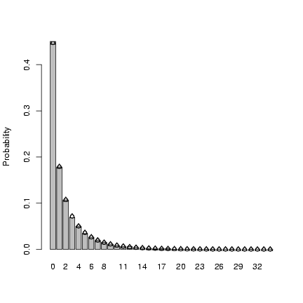
> mu = 2
> k = 0.5
> x = rnbinom(10000, mu = mu, size = k)
> tx = table(factor(x, levels = 0:max(x)))/10000
> b1 = barplot(tx, ylab = "Probability")
> points(b1, dnbinom(0:max(x), mu = mu, size = k), pch = 1)
> mean(x)
[1] 1.9445
> var(x)
[1] 9.585978
> mu
[1] 2
> mu * (1 + mu/k)
[1] 10
> p = 1/(1 + mu/k)
> n = k
> points(b1, dnbinom(0:max(x), prob = p, size = k), pch = 2)
 Here's how I translated p to n:
n=k and
Here's how I translated p to n:
n=k and
Exercise 3:
1.5 is the mean number of counts per category.
I suppose this could be interesting if you
were trying to describe an average sample size
per treatment, but otherwise it seems
pretty much irrelevant.
Exercise 4*:
Preliminaries: set up parameters and
derivative. Since we're only going to
be changing the distribution and not
the function, the second derivative
won't change.
> a = 0.696
> b = 9.79
> d1 = D(expression(a * x/(1 + (a/b) * x)), "x")
> d2 = D(d1, "x")
> Smean = 24.5
> d2_num = eval(d2, list(a = 0.696, b = 9.79, x = Smean))
> mval = a * Smean/(1 + (a/b) * Smean)
Solving for the parameters of the gamma in terms
of the moments
(m = as, s2=as2)
gives a=m2/s2, s=s2/m.
I'm going to build this into my function for
computing the integral.
> tmpf = function(S, mean = Smean, var) {
+     dgamma(S, shape = mean^2/var, scale = var/mean) * a * S/(1 +
+         (a/b) * S)
+ }
Check: I should the get the same answer as before when s2=m2=24.52
(which is true for the exponential distribution)
> integrate(tmpf, lower = 0, upper = Inf, var = Smean^2)
5.010691 with absolute error < 5.5e-05
Looks OK.
> Svar_vec = c(Smean^2, 100, 25, 1)
> dapprox = mval + 1/2 * Svar_vec * d2_num
> exact = c(integrate(tmpf, lower = 0, upper = Inf, var = Smean^2)$value,
+     integrate(tmpf, lower = 0, upper = Inf, var = 100)$value,
+     integrate(tmpf, lower = 0, upper = Inf, var = 25)$value,
+     integrate(tmpf, lower = 0, upper = Inf, var = 1)$value)
> merr = (mval - exact)/exact
> err = (dapprox - exact)/exact
> data.frame(exact = exact, mval = mval, delta = dapprox, mval.err = merr,
+     delta.err = err)
     exact     mval    delta     mval.err     delta.err
1 5.010691 6.219323 4.778299 0.2412106838 -4.637931e-02
2 5.983161 6.219323 5.979253 0.0394711611 -6.532386e-04
3 6.159482 6.219323 6.159306 0.0097153649 -2.858574e-05
4 6.216923 6.219323 6.216923 0.0003861181 -3.878837e-08
A slicker way to get all the exact values is:
> tmpf2 = function(var) {
+     integrate(tmpf, lower = 0, upper = Inf, var = var)$value
+ }
> sapply(Svar_vec, tmpf2)
[1] 5.010691 5.983161 6.159482 6.216923
Exercise 5*:
Based just on the expressions in the normalization constant
(G(a+b)/(G(a)G(b)) for the standard
parameterization, G(q)/(G(qP) G(q(1-P))))
gives q = a+b, P=a/(a+b)
or conversely a=qP, b=q(1-P).
In this parameterization, P is the mean proportion/
number of successes/etc. and q governs the width
of the distribution.
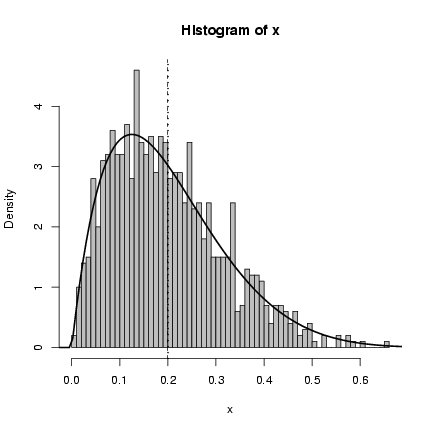
> my_rbeta = function(n, theta, P) {
+     rbeta(n, shape1 = theta * P, shape2 = theta * (1 - P))
+ }
> my_dbeta = function(x, theta, P) {
+     dbeta(x, shape1 = theta * P, shape2 = theta * (1 - P))
+ }
> x = my_rbeta(1000, theta = 10, P = 0.2)
> hist(x, breaks = 50, prob = TRUE, col = "gray")
> curve(my_dbeta(x, theta = 10, P = 0.2), add = TRUE, lwd = 2)
> abline(v = 0.2, lwd = 2, lty = 3)
> abline(v = mean(x), lty = 2)
 Exercise 6:
Define the functions:
Exercise 6:
Define the functions:
> dzinbinom = function(x, mu, size, zprob) {
+     ifelse(x == 0, zprob + (1 - zprob) * dnbinom(0, mu = mu,
+         size = size), (1 - zprob) * dnbinom(x, mu = mu, size = size))
+ }
> rzinbinom = function(n, mu, size, zprob) {
+     ifelse(runif(n) < zprob, 0, rnbinom(n, mu = mu, size = size))
+ }
Plotting (adding a point to show the fraction of the
zeros that come from sampling zeros):
> mu = 4
> size = 0.5
> zprob = 0.2
> x = rzinbinom(10000, mu = mu, size = size, zprob = zprob)
> tx = table(factor(x, levels = 0:max(x)))/10000
> b1 = barplot(tx, ylab = "Probability", ylim = c(0, 0.5))
> points(b1, dzinbinom(0:max(x), mu = mu, size = size, zprob = zprob),
+     pch = 16)
> points(b1[1], dnbinom(0, mu = mu, size = size) * (1 - zprob),
+     pch = 16, col = 2)
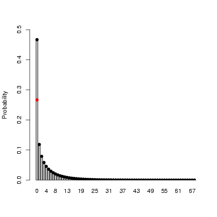 The mean of the zero-inflated negative binomial
is E[p·0 + (1-p) ·NegBin], or
(1-p times the mean of the negative binomial, or:
The mean of the zero-inflated negative binomial
is E[p·0 + (1-p) ·NegBin], or
(1-p times the mean of the negative binomial, or:
> mu * (1 - zprob)
[1] 3.2
> mean(x)
[1] 3.1405
Close enough ...
Exercise 7*:
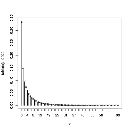
> mu = 4
> k = 0.5
> x = rpois(10000, rgamma(10000, shape = k, scale = mu/k))
> plot(table(x)/10000)
> points(0:max(x), dnbinom(0:max(x), mu = mu, size = k), cex = 0.75)
 Extra credit:
In order to get a lognormal with a specified mean
and variance, need to solve:
Extra credit:
In order to get a lognormal with a specified mean
and variance, need to solve:
for m and s.
Now substitute this value in for m in the second equation:
| |
|
|
e2(log(m)-s2/2) + s2 ·( es2 - 1 ) |
| |
| |
|
| |
| |
|
| |
| |
|
| |
| |
|
| |
| |
|
| |
| |
|
| |
|
Test this: if we start with m = 2.5, s2=3
(values picked haphazardly to test):
we get
> mu = 2.5
> sigmasq = 3
> m = exp(mu + sigmasq/2)
> v = exp(2 * mu + sigmasq) * (exp(sigmasq) - 1)
> s2 = log(v/m^2 + 1)
> s2
[1] 3
> m2 = log(m) - s2/2
> m2
[1] 2.5
Appears to work. Want a log-normal distribution
with the same mean and variance as the gamma distribution
that underlies the negative binomial with m = 4,
k=0.5. Since (shape) a=0.5, (scale) s=8, we have
mean=as=4 and var=as2=32.
> nsim = 1e+05
> s3 = log(32/4^2 + 1)
> s3
[1] 1.098612
> m3 = log(4) - s3/2
> m3
[1] 0.8369882
> lnormvals = rlnorm(nsim, meanlog = m3, sdlog = sqrt(s3))
> mean(lnormvals)
[1] 3.950413
> var(lnormvals)
[1] 31.08178
> poislnormvals = rpois(nsim, lnormvals)
Redraw:
> plot(table(factor(poislnormvals, levels = 0:max(poislnormvals)))/nsim,
+     xlim = c(0, 50))
> points(0:50, dnbinom(0:50, mu = mu, size = k), cex = 0.75, col = 2)
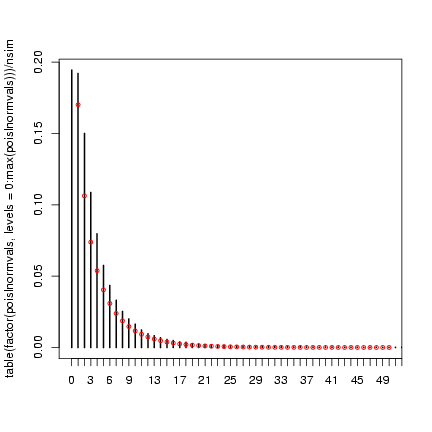 The lognormal-Poisson is actually (apparently) quite a different
shape, despite having the same mean and variance (this is more
apparent on a log scale):
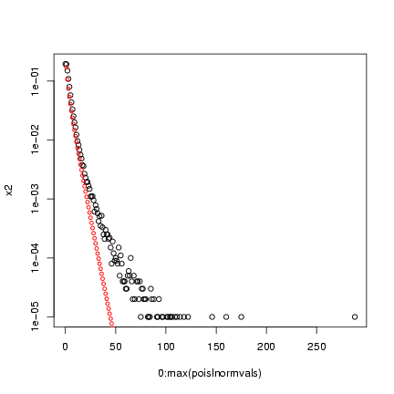
The lognormal-Poisson is actually (apparently) quite a different
shape, despite having the same mean and variance (this is more
apparent on a log scale):
> x2 = as.numeric(table(factor(poislnormvals, levels = 0:max(poislnormvals))))/nsim
> plot(0:max(poislnormvals), x2, log = "y")
> points(0:50, dnbinom(0:50, mu = mu, size = k), cex = 0.75, col = 2)
 Note that the variance of the compounded distribution is
(approximately) the variance of the underlying heterogeneity
plus the heterogeneity of the Poisson distribution
(which is equal to the mean of the Poisson).
Note that the variance of the compounded distribution is
(approximately) the variance of the underlying heterogeneity
plus the heterogeneity of the Poisson distribution
(which is equal to the mean of the Poisson).
> var(lnormvals)
[1] 31.08178
> var(poislnormvals)
[1] 34.65147
File translated from
TEX
by
TTH,
version 3.67.
On 28 Sep 2005, 13:39.