Lab 5: stochastic simulation - solutions
Ben Bolker
© 2005 Ben Bolker
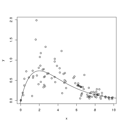
Exercise 1:
> n = 100
> x = runif(n, min = 0, max = 10)
> a = 1
> b = 0.5
> s = 3
> y_det = a * x * exp(-b * x)
> y = rgamma(n, shape = s, scale = y_det/s)
> plot(x, y)
> curve(a * x * exp(-b * x), add = TRUE)
 Exercise 2:
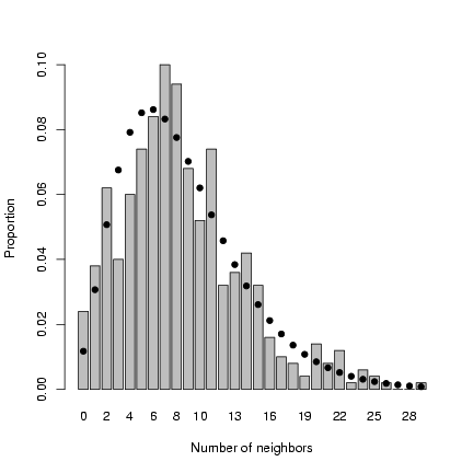
Redo spatial distribution simulation:
Exercise 2:
Redo spatial distribution simulation:
> set.seed(1001)
> nparents = 50
> noffspr = 10
> L = 30
> parent_x = runif(nparents, min = 0, max = L)
> parent_y = runif(nparents, min = 0, max = L)
> angle = runif(nparents * noffspr, min = 0, max = 2 * pi)
> dist = rexp(nparents * noffspr, 0.5)
> offspr_x = rep(parent_x, each = noffspr) + cos(angle) * dist
> offspr_y = rep(parent_y, each = noffspr) + sin(angle) * dist
> dist = sqrt((outer(offspr_x, offspr_x, "-"))^2 + (outer(offspr_y,
+     offspr_y, "-"))^2)
> nbrcrowd = apply(dist < 2, 1, sum) - 1
Calculate mean and standard deviation of neighborhood crowding:
> m = mean(nbrcrowd)
> s2 = var(nbrcrowd)
Method of moments: m = m;
variance s2=m(1+m/k)
or k = m/(s2/m-1).
> k.est = m/(s2/m - 1)
Plot distribution of neighborhood crowding:
> b1 = barplot(table(factor(nbrcrowd, levels = 0:max(nbrcrowd)))/length(nbrcrowd),
+     xlab = "Number of neighbors", ylab = "Proportion")
> points(b1, dnbinom(0:max(nbrcrowd), mu = m, size = k.est), pch = 16)
 Exercise 3:
Continue with pigweed simulation:
Exercise 3:
Continue with pigweed simulation:
> ci = nbrcrowd * 3
> M = 2.3
> alpha = 0.49
> mass_det = M/(1 + ci)
> mass = rgamma(length(mass_det), scale = mass_det, shape = alpha)
> b = 271.6
> k = 0.569
> seed_det = b * mass
> seed = rnbinom(length(seed_det), mu = seed_det, size = k)
Calculate the median: the median is identical
to the 50% quantile of the distribution,
or qnbinom(0.5).
> logxvec = seq(-7, 1, length = 100)
> xvec = 10^logxvec
> med = qnbinom(0.5, mu = b * xvec, size = k)
> plot(mass, 1 + seed, log = "xy", xlab = "Mass", ylab = "1+Seed set")
> curve(b * x + 1, add = TRUE)
> lower = qnbinom(0.025, mu = b * xvec, size = k)
> upper = qnbinom(0.975, mu = b * xvec, size = k)
> lines(xvec, lower + 1, lty = 2, type = "s")
> lines(xvec, upper + 1, lty = 2, type = "s")
> lines(xvec, med + 1, lwd = 2, type = "s")
 The median is lower than the mean because
the distribution is right-skewed; like the
upper and lower quantiles, the median of
the (discrete) negative binomial distribution changes
by discrete steps rather than smoothly like
the mean.
Exercise 4:
Set up simulation:
The median is lower than the mean because
the distribution is right-skewed; like the
upper and lower quantiles, the median of
the (discrete) negative binomial distribution changes
by discrete steps rather than smoothly like
the mean.
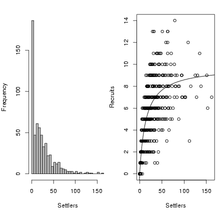
Exercise 4:
Set up simulation:
> rzinbinom = function(n, mu, size, zprob) {
+     ifelse(runif(n) < zprob, 0, rnbinom(n, mu = mu, size = size))
+ }
> a = 0.696
> b = 9.79
> recrprob = function(x, a = 0.696, b = 9.79) {
+     a/(1 + (a/b) * x)
+ }
> scoefs = c(mu = 25.32, k = 0.932, zprob = 0.123)
> settlers = rzinbinom(603, mu = scoefs["mu"], size = scoefs["k"],
+     zprob = scoefs["zprob"])
> recr = rbinom(603, prob = recrprob(settlers), size = settlers)
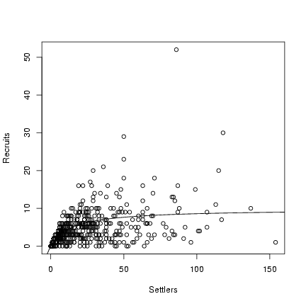
Draw the figure:
> op = par(mfrow = c(1, 2), mar = c(5, 4, 2, 0.2))
> hist(settlers, breaks = 40, col = "gray", ylab = "Frequency",
+     xlab = "Settlers", main = "")
> plot(settlers, recr, xlab = "Settlers", ylab = "Recruits")
> curve(a * x/(1 + (a/b) * x), add = TRUE)
> par(op)
 Exercise 5:
Using the relationships shape1=a=Pq and shape2=b=(1-P)q
relating the Morris (P, q) to the standard statistical parameterization:
Exercise 5:
Using the relationships shape1=a=Pq and shape2=b=(1-P)q
relating the Morris (P, q) to the standard statistical parameterization:
> rmbbinom = function(n, size, p, theta) {
+     rbinom(n, size = size, prob = rbeta(n, shape1 = p * theta,
+         shape2 = (1 - p) * theta))
+ }
> a = 0.696
> b = 9.79
> recrprob = function(x, a = 0.696, b = 9.79) a/(1 + (a/b) * x)
> scoefs = c(mu = 25.32, k = 0.932, zprob = 0.123)
> settlers = rzinbinom(603, mu = scoefs["mu"], size = scoefs["k"],
+     zprob = scoefs["zprob"])
> recr = rmbbinom(603, p = recrprob(settlers), theta = 10, size = settlers)
> plot(settlers, recr, xlab = "Settlers", ylab = "Recruits")
> curve(a * x/(1 + (a/b) * x), add = TRUE)
 Exercise 6:
Redefine linear simulation function:
Exercise 6:
Redefine linear simulation function:
> linsim = function(nt = 20, N0 = 2, dN = 1, sd_process = sqrt(2),
+     sd_obs = sqrt(2)) {
+     cur_N = N0
+     Nobs = numeric(nt)
+     Nobs[1] = cur_N + rnorm(1, sd = sd_obs)
+     for (i in 2:nt) {
+         cur_N = cur_N + rnorm(1, mean = dN, sd = sd_process)
+         Nobs[i] = cur_N + rnorm(1, sd = sd_obs)
+     }
+     return(Nobs)
+ }
Run it 1000 times:
> nsim = 1000
> Nmat = matrix(nrow = 20, ncol = nsim)
> for (i in 1:nsim) {
+     Nmat[, i] = linsim(sd_process = 2, sd_obs = 2)
+ }
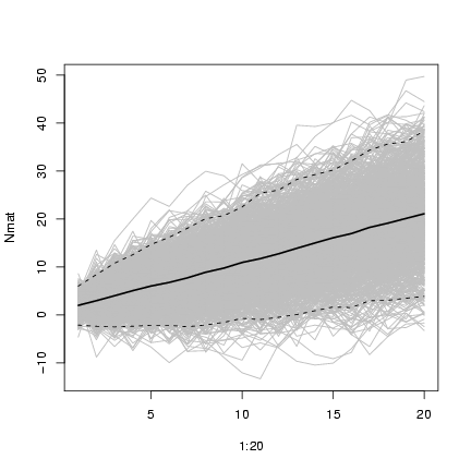
Draw the figure:
> matplot(1:20, Nmat, col = "gray", type = "l", lty = 1)
> lines(1:20, rowMeans(Nmat), lwd = 2)
> matlines(1:20, t(apply(Nmat, 1, quantile, c(0.025, 0.975))),
+     lty = 2, col = 1)
 Exercise 7:
Redefine immigsim with negative binomial instead of Poisson growth:
Exercise 7:
Redefine immigsim with negative binomial instead of Poisson growth:
> immignbsim = function(nt = 20, N0 = 2, immig, surv, k) {
+     N = numeric(nt)
+     N[1] = N0
+     for (i in 2:nt) {
+         Nsurv = rbinom(1, size = N[i - 1], prob = surv)
+         N[i] = Nsurv + rnbinom(1, mu = immig, size = k)
+     }
+     return(N)
+ }
Define parameters:
> nsim = 1000
> nt = 30
> p = 0.95
> N0 = 2
> immig = 10
> k = 0.5
> nvec = c(3, 5, 7, 10, 15, 20)
> kvec = c(5, 1, 0.5)
> nsim = 500
> powsimresults = matrix(nrow = length(nvec) * length(kvec) * nsim,
+     ncol = 6)
> colnames(powsimresults) = c("n", "k", "sim", "slope", "slope.lo",
+     "slope.hi")
> ctr = 1
> for (j in 1:length(kvec)) {
+     k = kvec[j]
+     for (i in 1:length(nvec)) {
+         nt = nvec[i]
+         tvec = 1:nt
+         for (sim in 1:nsim) {
+             current.sim = immignbsim(nt = nt, N0 = N0, surv = p,
+                 immig = immig, k = k)
+             lm1 = lm(current.sim ~ tvec)
+             slope = coef(lm1)["tvec"]
+             ci.slope = confint(lm1)["tvec", ]
+             powsimresults[ctr, ] = c(nt, k, sim, slope, ci.slope)
+             ctr = ctr + 1
+         }
+     }
+ }
Construct a list of factors for cross-tabulating:
> faclist = list(factor(powsimresults[, "n"]), factor(powsimresults[,
+     "k"]))
Calculate all the cross-tabulated summary statistics:
> slope.mean = tapply(powsimresults[, "slope"], faclist, mean)
> slope.sd = tapply(powsimresults[, "slope"], faclist, sd)
> ci.good = (powsimresults[, "slope.hi"] > immig) & (powsimresults[,
+     "slope.lo"] < immig)
> nsim = 500
> slope.cov = tapply(ci.good, faclist, sum)/nsim
> null.value = 0
> reject.null = (powsimresults[, "slope.hi"] < null.value) | (powsimresults[,
+     "slope.lo"] > null.value)
> slope.pow = tapply(reject.null, faclist, sum)/nsim
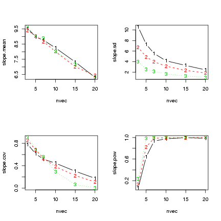
Some plots:
> par(mfrow = c(2, 2))
> matplot(nvec, slope.mean, type = "b")
> matplot(nvec, slope.sd, type = "b")
> matplot(nvec, slope.cov, type = "b")
> matplot(nvec, slope.pow, type = "b")
 Exercise 8:
Redo code with quadratic function, testing against a null value of zero:
Exercise 8:
Redo code with quadratic function, testing against a null value of zero:
> nvec = c(3, 5, 7, 10, 15, 20)
> nsim = 500
> powsimresults = matrix(nrow = length(nvec) * nsim, ncol = 5)
> colnames(powsimresults) = c("n", "sim", "quad", "quad.lo", "quad.hi")
> ctr = 1
> for (i in 1:length(nvec)) {
+     nt = nvec[i]
+     tvec = 1:nt
+     for (sim in 1:nsim) {
+         current.sim = immigsim(nt = nt, N0 = N0, surv = p, immig = immig)
+         lm1 = lm(current.sim ~ tvec + I(tvec^2))
+         quad = coef(lm1)[3]
+         ci.quad = confint(lm1)[3, ]
+         powsimresults[ctr, ] = c(nt, sim, quad, ci.quad)
+         ctr = ctr + 1
+     }
+ }
Calculate all the tabulated summary statistics (skipping coverage):
> quad.mean = tapply(powsimresults[, "quad"], nfac, mean)
> quad.sd = tapply(powsimresults[, "quad"], nfac, sd)
> nsim = 500
> null.value = 0
> reject.null = (powsimresults[, "quad.hi"] < null.value) | (powsimresults[,
+     "quad.lo"] > null.value)
> quad.pow = tapply(reject.null, nfac, sum)/nsim
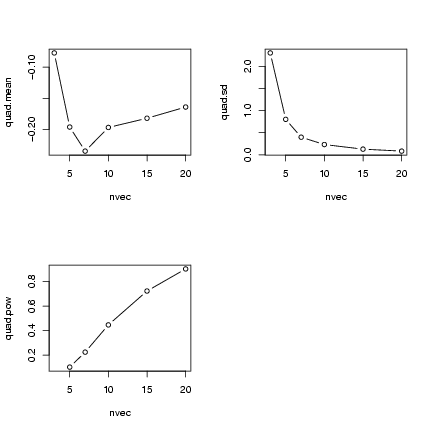
Some plots:
> op = par(mfrow = c(2, 2))
> plot(nvec, quad.mean, type = "b")
> plot(nvec, quad.sd, type = "b")
> plot(nvec, quad.pow, type = "b")
> par(op)
File translated from
TEX
by
TTH,
version 3.67.
On 7 Oct 2005, 11:39.