Contents
function out = keen_2000()
close all
clc
warning on
Parameters attribution and function definitions
par_alpha = 0.025;
par_beta = 0.02;
par_gamma = 0.01;
par_nu = 3;
par_r = 0.03;
par_A = -57.911;
par_B = 56.162;
par_C = -0.00956;
fun_Phi = @(x) exp(par_A+par_B.*x)+par_C;
fun_Phi_inv = @(y) (log(y-par_C)-par_A)./par_B;
par_A_mod = 0.0000641;
par_B_mod = 1;
par_C_mod = 0.0400641
fun_Phi_mod = @(x) par_A_mod./(par_B_mod-x).^2- par_C_mod;
fun_Phi_mod_inv = @(y) par_B_mod - sqrt(par_A_mod./(y+par_C_mod));
par_D = -5 ;
par_E = 20;
par_F = -0.0065;
fun_kappa = @(x) min(1,exp(par_D+par_E.*x)+par_F);
fun_kappa_inv = @(y) (log(y-par_F)-par_D)./par_E;
par_G = 13.5;
par_H = -18.5;
par_I = -0.018;
fun_Gamma = @(x) exp(par_G+par_H*x)+par_I;
par_J = -4.465;
par_K = 8.368;
par_L = -0.027;
fun_Theta = @(x) exp(par_J+par_K*x)+par_L;
TOL = 1E-7;
options = odeset('RelTol', TOL);
txt_format = '%3.3g';
par_C_mod =

    0.0401
Perturbation analysis, page 93
lambda_eq = fun_Phi_inv(par_alpha)
pi_eq = fun_kappa_inv(par_nu*(par_alpha+par_beta+par_gamma))
d_eq = (par_nu*(par_alpha+par_beta+par_gamma)-pi_eq)/(par_alpha+par_beta)
omega_eq = 1-pi_eq-par_r*d_eq
omega0 = 0.81;
lambda0 = 0.94;
d0 = 0.04;
y0 = [convert([omega0, lambda0]),d0];
T = 80;
par1 = [par_nu,par_alpha,par_beta,par_gamma,par_r,par_A,par_B,par_C,par_D,par_E,par_F];
[tK,yK] = ode15s(@(t,y) keen(y,par1), [0 T], y0, options);
yKnew = retrieve([yK(:,1),yK(:,2)]);
yK(:,1) = yKnew(:,1);
yK(:,2) = yKnew(:,2);
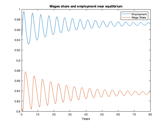
figure(1)
plot(tK, yK(:,2),tK,yK(:,1))
xlabel('Years')
legend('Employment','Wage Share')
title(['Wages share and employment near equilibrium'])
figure(2)
plot(tK, yK(:,3))
xlabel('Years')
ylabel('Debt to output ratio')
title(['Debt-to-output ratio near equilibrium'])
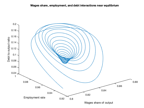
figure(3)
plot3(yK(:,1),yK(:,2),yK(:,3))
xlabel('Wages share of output')
ylabel('Employment rate')
zlabel('Debt to output ratio')
title(['Wages share, employment, and debt interactions near equilibrium'])
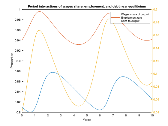
figure(4)
N=max(find(tK<=10));
plot(tK(1:N), yK(1:N,1),tK(1:N),yK(1:N,2))
xlabel('Years')
ylabel('Proportion')
yyaxis('right')
ylabel('Debt-to-output ratio')
plot(tK(1:N), yK(1:N,3))
legend('Wages share of output','Employment rate','Debt-to-output')
title(['Period interactions of wages share, employment, and debt near equilibrium'])
lambda_eq_mod = fun_Phi_mod_inv(par_alpha);
omega0 = omega_eq-0.11;
lambda0 = lambda_eq_mod-0.05;
d0 = d_eq;
y0 = [convert([omega0, lambda0]),d0];
T = 100;
par2_mod = [par_nu,par_alpha,par_beta,par_gamma,par_r,par_A_mod,par_B_mod,par_C_mod,par_D,par_E,par_F];
[tK,yK] = ode15s(@(t,y) keen_mod(y,par2_mod), [0 T], y0, options);
yKnew = retrieve([yK(:,1),yK(:,2)]);
yK(:,1) = yKnew(:,1);
yK(:,2) = yKnew(:,2);
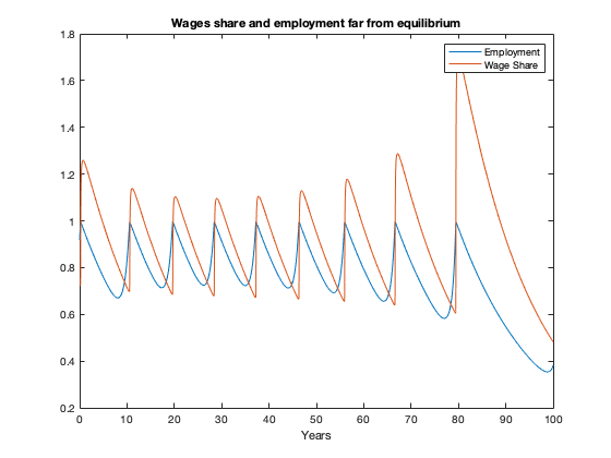
figure(5)
plot(tK, yK(:,2),tK,yK(:,1))
xlabel('Years')
legend('Employment','Wage Share')
title(['Wages share and employment far from equilibrium'])
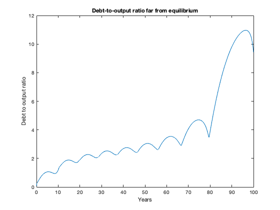
figure(6)
plot(tK, yK(:,3))
xlabel('Years')
ylabel('Debt to output ratio')
title(['Debt-to-output ratio far from equilibrium'])
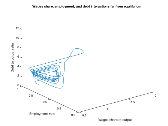
figure(7)
plot3(yK(:,1),yK(:,2),yK(:,3))
xlabel('Wages share of output')
ylabel('Employment rate')
zlabel('Debt to output ratio')
title(['Wages share, employment, and debt interactions far from equilibrium'])
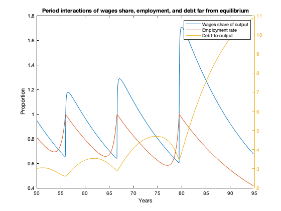
figure(8)
N_min=min(find(tK>50));
N_max=max(find(tK<=95));
plot(tK(N_min:N_max), yK(N_min:N_max,1),tK(N_min:N_max),yK(N_min:N_max,2))
xlabel('Years')
ylabel('Proportion')
yyaxis('right')
ylabel('Debt-to-output ratio')
plot(tK(N_min:N_max), yK(N_min:N_max,3))
legend('Wages share of output','Employment rate','Debt-to-output')
title(['Period interactions of wages share, employment, and debt far from equilibrium'])
lambda_eq =

    0.9712


pi_eq =

    0.1618


d_eq =

    0.0702


omega_eq =

    0.8361

Adding a government sector, page 100
par3_mod = [par_nu,par_alpha,par_beta,par_gamma,par_r,par_A_mod,par_B_mod,par_C_mod,par_D,par_E,par_F...
par_G,par_H,par_I,par_J,par_K,par_L];
lambda_eq = fun_Phi_inv(par_alpha)
pi_eq = fun_kappa_inv(par_nu*(par_alpha+par_beta+par_gamma))
g_eq = fun_Gamma(lambda_eq)/(par_alpha+par_beta)
t_eq = fun_Theta(pi_eq)/(par_alpha+par_beta)
d_eq = (par_nu*(par_alpha+par_beta+par_gamma)-pi_eq)/(par_alpha+par_beta)
omega_eq = 1-pi_eq-par_r*d_eq-t_eq+g_eq
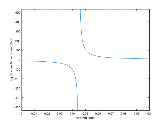
d_g_eq=(t_eq-g_eq)/(par_r-par_alpha-par_beta)
figure(9)
z=[];
syms d_g(z)
d_g(z) = (t_eq-g_eq)/(z-par_alpha-par_beta);
fplot(d_g,[0,0.1]);
xlabel('Interest Rate')
ylabel('Equilibrium Government Debt')
omega0 = 0.31;
lambda0 = 0.98;
dk0 = 0.08;
dg0 = -36;
g0 = -0.13;
t0 = 0.4;
y0 = [convert([omega0, lambda0]),dk0,dg0,g0,t0];
T = 200;
[tK,yK] = ode15s(@(t,y) keen_government(y,par3_mod), [0 T], y0, options);
yKnew = retrieve([yK(:,1),yK(:,2)]);
yK(:,1) = yKnew(:,1);
yK(:,2) = yKnew(:,2);
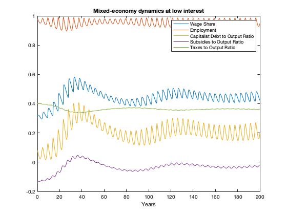
figure(10)
plot(tK, yK(:,1),tK,yK(:,2),tK,yK(:,3),tK,yK(:,5),tK,yK(:,6))
xlabel('Years')
legend('Wage Share','Employment','Capitalist Debt to Output Ratio','Subsidies to Output Ratio','Taxes to Output Ratio')
title(['Mixed-economy dynamics at low interest'])
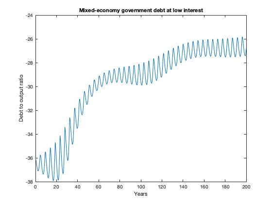
figure(11)
plot(tK, yK(:,4))
xlabel('Years')
ylabel('Debt to output ratio')
title(['Mixed-economy government debt at low interest'])
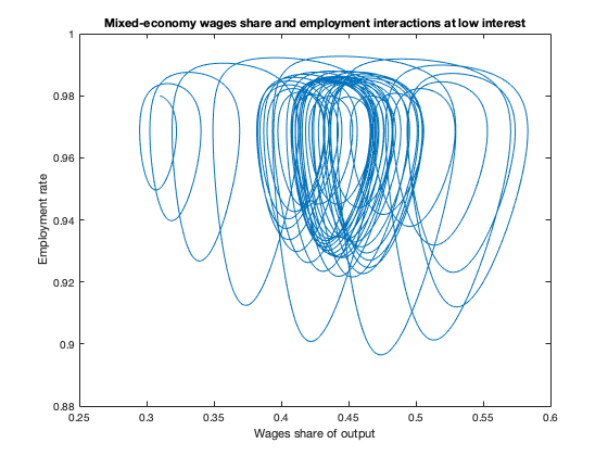
figure(12)
plot(yK(:,1),yK(:,2))
xlabel('Wages share of output')
ylabel('Employment rate')
title(['Mixed-economy wages share and employment interactions at low interest'])
par_r = 0.05;
par4_mod = [par_nu,par_alpha,par_beta,par_gamma,par_r,par_A_mod,par_B_mod,par_C_mod,par_D,par_E,par_F...
par_G,par_H,par_I,par_J,par_K,par_L];
omega0 = 0.31;
lambda0 = 0.98;
dk0 = 0.08;
dg0 = 110;
g0 = -0.13;
t0 = 0.4;
y0 = [convert([omega0, lambda0]),dk0,dg0,g0,t0];
T = 200;
[tK,yK] = ode15s(@(t,y) keen_government(y,par4_mod), [0 T], y0, options);
yKnew = retrieve([yK(:,1),yK(:,2)]);
yK(:,1) = yKnew(:,1);
yK(:,2) = yKnew(:,2);
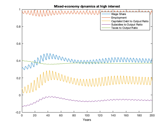
figure(13)
plot(tK, yK(:,1),tK,yK(:,2),tK,yK(:,3),tK,yK(:,5),tK,yK(:,6))
xlabel('Years')
legend('Wage Share','Employment','Capitalist Debt to Output Ratio','Subsidies to Output Ratio','Taxes to Output Ratio')
title(['Mixed-economy dynamics at high interest'])
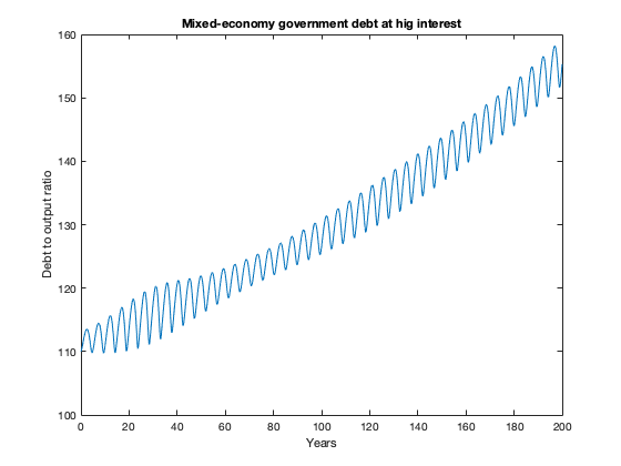
figure(14)
plot(tK, yK(:,4))
xlabel('Years')
ylabel('Debt to output ratio')
title(['Mixed-economy government debt at hig interest'])
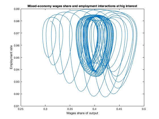
figure(15)
plot(yK(:,1),yK(:,2))
xlabel('Wages share of output')
ylabel('Employment rate')
title(['Mixed-economy wages share and employment interactions at hig interest'])
lambda_eq =

    0.9712


pi_eq =

    0.1618


g_eq =

   -0.1450


t_eq =

    0.3904


d_eq =

    0.0702


omega_eq =

    0.3006


d_g_eq =

  -35.6965
Auxiliary functions
function new = convert(old,r)
n = size(old,2);
new = zeros(size(old));
new(:,1) = log(old(:,1));
new(:,2) = tan((old(:,2)-0.5)*pi);
if n>2
new(:,3) = 1-old(:,1)-r*old(:,3);
if n==4
new(:,4) = log(old(:,4));
end
end
end
function old = retrieve(new,r)
n = size(new,2);
old = zeros(size(new));
old(:,1) = exp(new(:,1));
old(:,2) = atan(new(:,2))/pi+0.5;
if n>2
old(:,3) = (1-old(:,1)-new(:,3))/r;
if n==4
old(:,4) = exp(new(:,4));
end
end
end
function f = keen(y,par)
f = zeros(3,1);
log_omega = y(1);
tan_lambda = y(2);
d = y(3);
lambda = atan(tan_lambda)/pi+0.5;
omega = exp(log_omega);
nu = par(1);
alpha = par(2);
beta = par(3);
gamma = par(4);
r = par(5);
A = par(6);
B = par(7);
C = par(8);
D = par(9);
E = par(10);
F = par(11);
pi_n = 1-omega-r*d;
phillips = exp(A+B*lambda)+C;
kappa = exp(D+E*pi_n)+F;
g_Y = kappa/nu-gamma;
f(1) = phillips-alpha;
f(2) = (1+tan_lambda^2)*pi*lambda*(g_Y-alpha-beta);
f(3) = d*(r-(kappa/nu-gamma))+kappa-(1-omega);
end
function f = keen_mod(y,par)
f = zeros(3,1);
log_omega = y(1);
tan_lambda = y(2);
d = y(3);
lambda = atan(tan_lambda)/pi+0.5;
omega = exp(log_omega);
nu = par(1);
alpha = par(2);
beta = par(3);
gamma = par(4);
r = par(5);
A = par(6);
B = par(7);
C = par(8);
D = par(9);
E = par(10);
F = par(11);
pi_n = 1-omega-r*d;
phillips = A./(B-lambda)^2- C;
kappa = exp(D+E*pi_n)+F;
g_Y = kappa/nu-gamma;
f(1) = phillips-alpha;
f(2) = (1+tan_lambda^2)*pi*lambda*(g_Y-alpha-beta);
f(3) = d*(r-(kappa/nu-gamma))+kappa-(1-omega);
end
function f = keen_government(y,par)
f = zeros(6,1);
log_omega = y(1);
tan_lambda = y(2);
dk = y(3);
dg = y(4);
g = y(5);
t = y(6);
lambda = atan(tan_lambda)/pi+0.5;
omega = exp(log_omega);
nu = par(1);
alpha = par(2);
beta = par(3);
gamma = par(4);
r = par(5);
A = par(6);
B = par(7);
C = par(8);
D = par(9);
E = par(10);
F = par(11);
G = par(12);
H = par(13);
I = par(14);
J = par(15);
K = par(16);
L = par(17);
pi_n = 1-omega-r.*dk+g-t;
phillips = A./(B-lambda)^2- C;
kappa = exp(D+E*pi_n)+F;
Gamma = exp(G+H*lambda)+I;
Theta = exp(J+K*pi_n)+L;
g_Y = kappa/nu-gamma;
f(1) = phillips-alpha;
f(2) = (1+tan_lambda^2)*pi*lambda*(g_Y-alpha-beta);
f(3) = kappa-(1-omega)+t-g+dk*(r-kappa/nu+gamma);
f(4) = dg*(r-kappa/nu+gamma)+g-t;
f(5) = Gamma - g*(kappa/nu-gamma);
f(6) = Theta - t*(kappa/nu-gamma);
end
end