Contents
- Base Parameters - Table 2
- Other definitions
- Functions of interest
- Example 1: good equilibirum of Keen model without policy rate
- Example 2: bad equilibrium of Keen model without policy rate
- Example 3: good equilibrium with policy rate
- Example 4: stabilizaing policy rate with high debt levels
- Example 5: stabilizaing policy rate with higher debt levels
- Auxiliary functions
function out = negative_paper()
%%%%%%%%%%%%%%%%%%%%%%%%%%%%%%%%%%%%%%%%%%%%%%%%%%%%%%%%%%%%%%%%%%%%%%%%%%%
% This code simulates the Keen model with monetary policy as
% specified in Grasselli and Lipton (2019)
%
% authors: M. Grasselli and A. Lipton
%%%%%%%%%%%%%%%%%%%%%%%%%%%%%%%%%%%%%%%%%%%%%%%%%%%%%%%%%%%%%%%%%%%%%%%%%%%
close all
clc
warning off
Base Parameters - Table 2
a = -0.0401;    % constant parameter in phillips curve
b_phil = 0.0001;% coefficient phillips curve
c = -0.0065;    % constant parameter in investment function
d_i = -5;         % affine parameter in exponent of investment function
e = 20;         % coefficient in the exponent of investment function
kr= 0.1;        % capital ratio for banks (loan/equity)
markup = 1.3;   % markup factor
alpha = 0.025;  % growth rate in productivity
beta =0.02;     % growth rate in population
gamma=0.8;      % money illusion coefficient
delta=0.03;     % depreciation rate
etap=0.35;      % inflation relaxation parameter
nu=3;           % capital to output ratio
Other definitions
TOL = 1E-7;
options = odeset('RelTol', TOL);
txt_format = '%3.3g';
Functions of interest
inflation = @(x) etap*(markup*x-1);              % inflation, equation (10)

phillips = @(x) a+b_phil./(1-x).^2;                  % Phillips curve, equation (24)

investment= @(x) c+exp(d_i+e.*x);                 % investment function, equation (25)
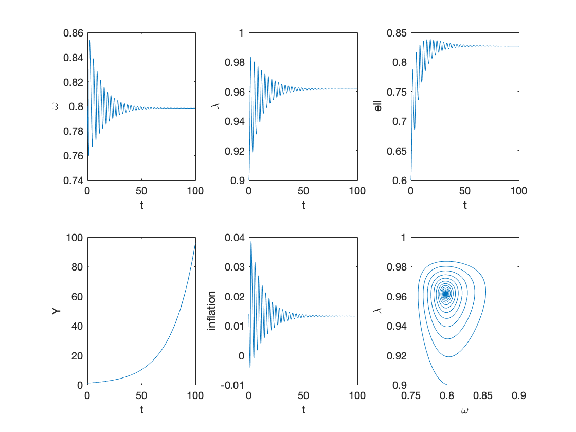
Example 1: good equilibirum of Keen model without policy rate
tax=0;        % tax to income ratio
g=0;          % government spending to income ratio
etag=0;       % speed of adjustment of rho
etar=0;       % speed of adjustment of rg
deltar=0.03;  % interest rate spread

T=100;

omega0=0.8;
lambda0=0.9;
l0=0.6;
rho0=0;
rg0=0;
b0=0;
Y0=1;

y0=[convert([omega0,lambda0]),l0,rho0,rg0,b0];

[tK,yK] = ode15s(@(t,y) main(y), [0 T], y0, options);
sol = retrieve([yK(:,1),yK(:,2)]);
yK(:,1)=sol(:,1);
yK(:,2)=sol(:,2);
Y_output = Y0*yK(:,2)/lambda0.*exp((alpha+beta)*tK);


% Figure 2
figure
subplot(2,3,1)
plot(tK,yK(:,1))
xlabel('t')
ylabel('\omega')

subplot(2,3,2)
plot(tK,yK(:,2))
xlabel('t')
ylabel('\lambda')

subplot(2,3,3)
plot(tK,yK(:,3))
xlabel('t')
ylabel('ell')

subplot(2,3,4)
plot(tK,Y_output)
xlabel('t')
ylabel('Y')

inflation_sol=inflation(yK(:,1));
subplot(2,3,5)
plot(tK,inflation_sol)
xlabel('t')
ylabel('inflation')

subplot(2,3,6)
plot(yK(:,1),yK(:,2))
xlabel('\omega')
ylabel('\lambda')
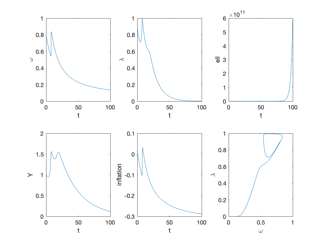
Example 2: bad equilibrium of Keen model without policy rate
tax=0;        % tax to income ratio
g=0;          % government spending to income ratio
etag=0;       % speed of adjustment of rho
etar=0;       % speed of adjustment of rg
deltar=0.03;  % interest rate spread

T=100;

omega0=0.8;
lambda0=0.9;
l0=6;         % NOTE: this is incorrectly listed in the paper as l0 = 0.6
rho0=0;
rg0=0;
b0=0;
Y0=1;

y0=[convert([omega0,lambda0]),l0,rho0,rg0,b0];

[tK,yK] = ode15s(@(t,y) main(y), [0 T], y0, options);
sol = retrieve([yK(:,1),yK(:,2)]);
yK(:,1)=sol(:,1);
yK(:,2)=sol(:,2);
Y_output = Y0*yK(:,2)/lambda0.*exp((alpha+beta)*tK);

% Figure 3
figure
subplot(2,3,1)
plot(tK,yK(:,1))
xlabel('t')
ylabel('\omega')

subplot(2,3,2)
plot(tK,yK(:,2))
xlabel('t')
ylabel('\lambda')

subplot(2,3,3)
plot(tK,yK(:,3))
xlabel('t')
ylabel('ell')

subplot(2,3,4)
plot(tK,Y_output)
xlabel('t')
ylabel('Y')

inflation_sol=inflation(yK(:,1));
subplot(2,3,5)
plot(tK,inflation_sol)
xlabel('t')
ylabel('inflation')

subplot(2,3,6)
plot(yK(:,1),yK(:,2))
xlabel('\omega')
ylabel('\lambda')
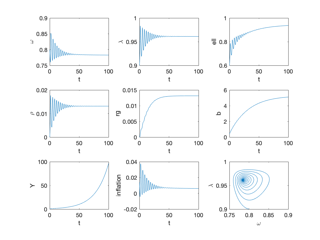
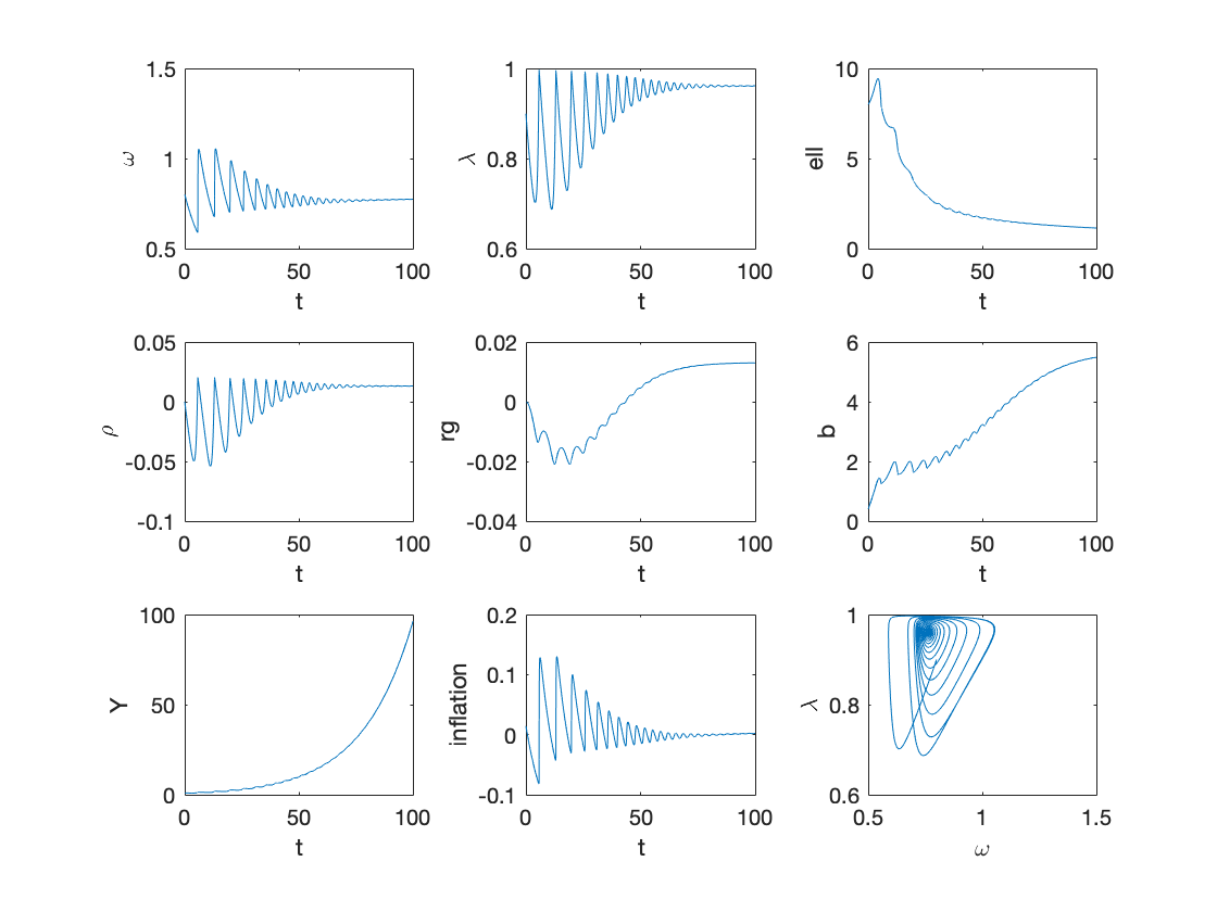
Example 3: good equilibrium with policy rate
tax=0;        % tax to income ratio
g=0.2;          % government spending to income ratio
etag=0.2;       % speed of adjustment of rho
etar=0.1;       % speed of adjustment of rg
deltar=0.03;  % interest rate spread

T=100;

omega0=0.8;
lambda0=0.9;
l0=0.6;
rho0=0;
rg0=0;
b0=0.4;
Y0=1;

y0=[convert([omega0,lambda0]),l0,rho0,rg0,b0];

[tK,yK] = ode15s(@(t,y) main(y), [0 T], y0, options);
sol = retrieve([yK(:,1),yK(:,2)]);
yK(:,1)=sol(:,1);
yK(:,2)=sol(:,2);
Y_output = Y0*yK(:,2)/lambda0.*exp((alpha+beta)*tK);

% Figure 4
figure
subplot(3,3,1)
plot(tK,yK(:,1))
xlabel('t')
ylabel('\omega')

subplot(3,3,2)
plot(tK,yK(:,2))
xlabel('t')
ylabel('\lambda')

subplot(3,3,3)
plot(tK,yK(:,3))
xlabel('t')
ylabel('ell')

subplot(3,3,4)
plot(tK,yK(:,4))
xlabel('t')
ylabel('\rho')

subplot(3,3,5)
plot(tK,yK(:,5))
xlabel('t')
ylabel('rg')

subplot(3,3,6)
plot(tK,yK(:,6))
xlabel('t')
ylabel('b')

subplot(3,3,7)
plot(tK,Y_output)
xlabel('t')
ylabel('Y')

inflation_sol=inflation(yK(:,1));
subplot(3,3,8)
plot(tK,inflation_sol)
xlabel('t')
ylabel('inflation')

subplot(3,3,9)
plot(yK(:,1),yK(:,2))
xlabel('\omega')
ylabel('\lambda')
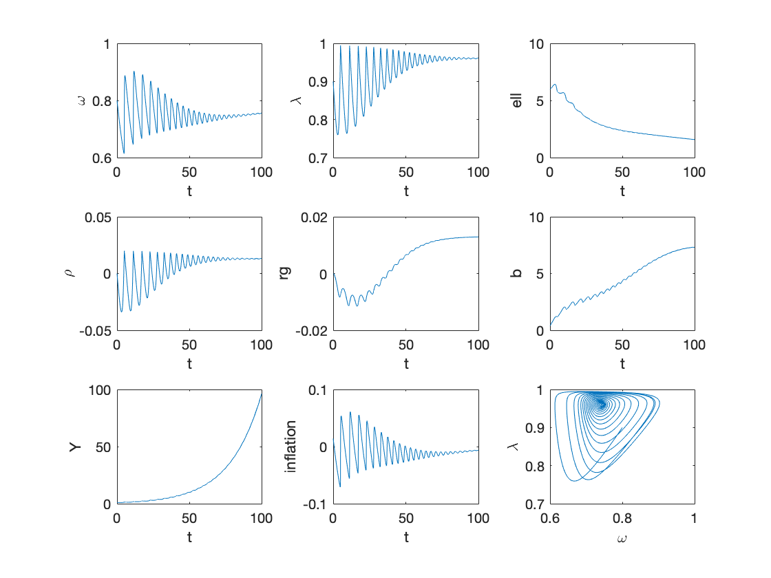
Example 4: stabilizaing policy rate with high debt levels
tax=0;        % tax to income ratio
g=0.2;          % government spending to income ratio
etag=0.2;       % speed of adjustment of rho
etar=0.1;       % speed of adjustment of rg
deltar=0.03;  % interest rate spread

T=100;

omega0=0.8;
lambda0=0.9;
l0=6;
rho0=0;
rg0=0;
b0=0.4;
Y0=1;

y0=[convert([omega0,lambda0]),l0,rho0,rg0,b0];

[tK,yK] = ode15s(@(t,y) main(y), [0 T], y0, options);
sol = retrieve([yK(:,1),yK(:,2)]);
yK(:,1)=sol(:,1);
yK(:,2)=sol(:,2);
Y_output = Y0*yK(:,2)/lambda0.*exp((alpha+beta)*tK);

% Figure 5
figure
subplot(3,3,1)
plot(tK,yK(:,1))
xlabel('t')
ylabel('\omega')

subplot(3,3,2)
plot(tK,yK(:,2))
xlabel('t')
ylabel('\lambda')

subplot(3,3,3)
plot(tK,yK(:,3))
xlabel('t')
ylabel('ell')

subplot(3,3,4)
plot(tK,yK(:,4))
xlabel('t')
ylabel('\rho')

subplot(3,3,5)
plot(tK,yK(:,5))
xlabel('t')
ylabel('rg')

subplot(3,3,6)
plot(tK,yK(:,6))
xlabel('t')
ylabel('b')

subplot(3,3,7)
plot(tK,Y_output)
xlabel('t')
ylabel('Y')

inflation_sol=inflation(yK(:,1));
subplot(3,3,8)
plot(tK,inflation_sol)
xlabel('t')
ylabel('inflation')

subplot(3,3,9)
plot(yK(:,1),yK(:,2))
xlabel('\omega')
ylabel('\lambda')
Example 5: stabilizaing policy rate with higher debt levels
tax=0;          % tax to income ratio
g=0.2;          % government spending to income ratio
etag=0.2;       % speed of adjustment of rho
etar=0.1;       % speed of adjustment of rg
deltar=0.03;    % interest rate spread

T=100;

omega0=0.8;
lambda0=0.9;
l0=8;
rho0=0;
rg0=0;
b0=0.4;
Y0=1;

y0=[convert([omega0,lambda0]),l0,rho0,rg0,b0];

[tK,yK] = ode15s(@(t,y) main(y), [0 T], y0, options);
sol = retrieve([yK(:,1),yK(:,2)]);
yK(:,1)=sol(:,1);
yK(:,2)=sol(:,2);
Y_output = Y0*yK(:,2)/lambda0.*exp((alpha+beta)*tK);

% Figure 6
figure
subplot(3,3,1)
plot(tK,yK(:,1))
xlabel('t')
ylabel('\omega')

subplot(3,3,2)
plot(tK,yK(:,2))
xlabel('t')
ylabel('\lambda')

subplot(3,3,3)
plot(tK,yK(:,3))
xlabel('t')
ylabel('ell')

subplot(3,3,4)
plot(tK,yK(:,4))
xlabel('t')
ylabel('\rho')

subplot(3,3,5)
plot(tK,yK(:,5))
xlabel('t')
ylabel('rg')

subplot(3,3,6)
plot(tK,yK(:,6))
xlabel('t')
ylabel('b')

subplot(3,3,7)
plot(tK,Y_output)
xlabel('t')
ylabel('Y')

inflation_sol=inflation(yK(:,1));
subplot(3,3,8)
plot(tK,inflation_sol)
xlabel('t')
ylabel('inflation')

subplot(3,3,9)
plot(yK(:,1),yK(:,2))
xlabel('\omega')
ylabel('\lambda')
Auxiliary functions
Instead of integrating the system in terms of omega, lambda and d, we decided to use:
log_omega = log(omega), tan_lambda = tan((lambda-0.5)*pi)
Experiments show that the numerical methods work better with these variables.
function new = convert(old)
    % This function converts
    % [omega, lambda]
    % to
    % [log_omega, tan_lambda]


    n = size(old,2); %number of variables
    new = zeros(size(old));

    new(:,1) = log(old(:,1));
    new(:,2) = tan((old(:,2)-0.5)*pi);
end

function old = retrieve(new)
    % This function retrieves [omega, lambda]
    % from
    % [log_omega, tan_lambda]

    n = size(new,2); %number of variables
    old = zeros(size(new));

    old(:,1) = exp(new(:,1));
    old(:,2) = atan(new(:,2))/pi+0.5;
end

function f = main(y)    % solves the main dynamical system
    f = zeros(6,1);

    log_omega = y(1);
    tan_lambda = y(2);
    l = y(3);
    rho= y(4);
    rg=y(5);
    b=y(6);

    lambda = atan(tan_lambda)/pi+0.5;
    omega = exp(log_omega);
    profit = 1-omega-tax-(rg+deltar)*l;

    growth = investment(profit)/nu-delta;    % real growth rate

    % Equation (13)
    f(1) = phillips(lambda)-(1-gamma)*inflation(omega)-alpha; %d(log_omega)/dt
    f(2) = (1+tan_lambda^2)*pi*lambda*(growth-alpha-beta); %d(tan_lambda)/dt
    f(3) = (rg+deltar-growth-inflation(omega))*l+omega+tax+investment(profit)-1; %d(l)/dt
    f(4) = etag*(growth-alpha-beta);     %d(rho)/dt
    f(5) = etar*(rho-rg);                %d(rg)/dt

    % Equation (18)
    f(6) = (g-tax)+b*(rg-inflation(omega)-growth);   %db/dt

end
end