Contents
function out = two_class_dual_keen()
%%%%%%%%%%%%%%%%%%%%%%%%%%%%%%%%%%%%%%%%%%%%%%%%%%%%%%%%%%%%%%%%%%%%%%%%%%%
% This code simulates the dual Keen model with two classes of
% households as specified in Giraud and Grasselli (2019)
%
%
% authors: G. Giraud and M. Grasselli
%%%%%%%%%%%%%%%%%%%%%%%%%%%%%%%%%%%%%%%%%%%%%%%%%%%%%%%%%%%%%%%%%%%%%%%%%%%
clear all
close all
clc
warning off
Base Parameters - Table 3 (modified for two classes)
nu = 3;          %capital to output ratio
alpha = 0.025;   %productivity growth rate
beta = 0.02;     %population growth rate
delta = 0.05;    %depreciation rate
r = 0.03;        %real interest rate
eta_p = 0.35;    % adjustment speed for prices
markup = 1.6;    % mark-up value
gamma = 0.8;     % (1-gamma) is the degree of money ilusion
theta = 0.2; % proportion of profits paid to investors - MODIFIED

phi0 = 0.04/(1-0.04^2); %Phillips curve parameter
phi1 = 0.04^3/(1-0.04^2); %Phillips curve parameter
 c_minus_w = 0.02; % consumption share hard-lower bound for workers - MODIFIED
 c_minus_i = 0.01; % consumption share hard-lower bound for investors - MODIFIED
 A_c = 0; %Consumption share asymptotic lower bound
 B_c = 5; % Consumption share growth rate
 C_c = 1;
 K_w = 0.75; % Consumption share upper bound for workers - MODIFIED
 K_i = 0.15; % Consumption share upper bound for investors - MODIFED
 nu_c = 0.2;
 Q_w= ((K_w-A_c)/(c_minus_w-A_c))^nu_c-C_c;
 Q_i= ((K_i-A_c)/(c_minus_i-A_c))^nu_c-C_c;

% Other definitions
TOL = 1E-7;
options = odeset('RelTol', TOL);
txt_format = '%3.3g';
Functions of interest
fun_consumption_w =@(x) max(c_minus_w,A_c + ((K_w-A_c)./(C_c+Q_w*exp(-B_c*x)).^(1/nu_c))); %----first specification : generalised logistic consumption function------%
fun_consumption_w_inv = @(x) -log((((K_w-A_c)./(x-A_c)).^nu_c-C_c)./Q_w)./B_c; % inverse of the consumption function over positive income

fun_consumption_i =@(x) max(c_minus_i,A_c + ((K_i-A_c)./(C_c+Q_i*exp(-B_c*x)).^(1/nu_c))); %----first specification : generalised logistic consumption function------%
fun_consumption_i_inv = @(x) -log((((K_i-A_c)./(x-A_c)).^nu_c-C_c)./Q_i)./B_c; % inverse of the consumption function over positive income

total_consumption =@(x) fun_consumption_w(x)+fun_consumption_i(x);

fun_Phi = @(x) phi1./(1-x).^2- phi0;
fun_Phi_prime = @(x) 2*phi1./(1-x).^3;
fun_Phi_inv = @(x) 1 - (phi1./(x+phi0)).^(1/2);
Example 1
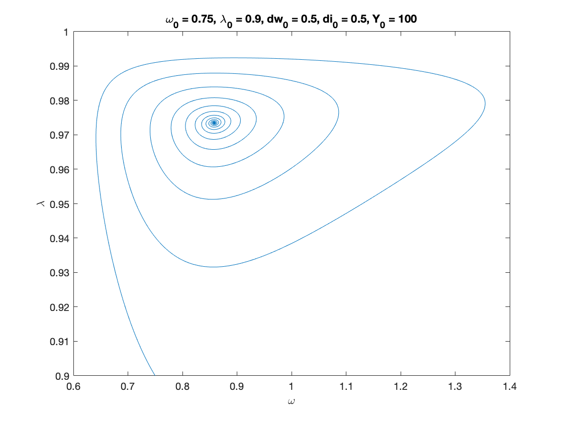
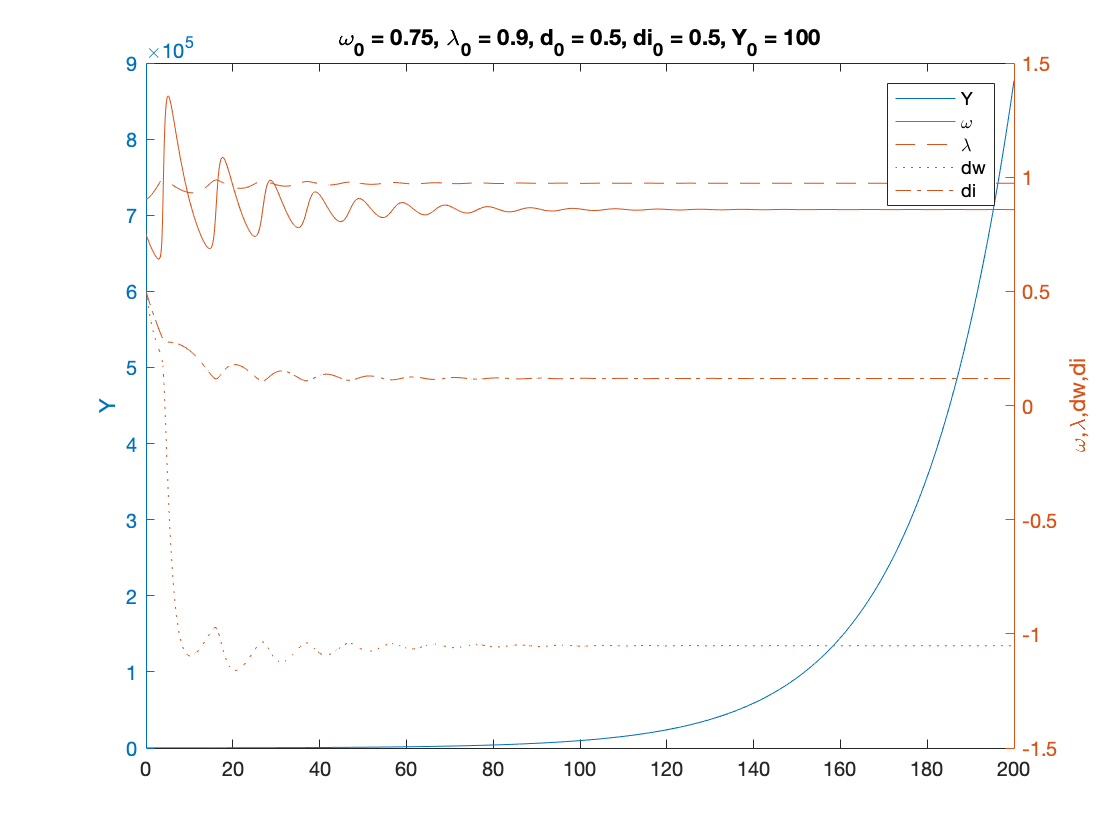
% Parameters as in Table 3 (modified for two classes)

nu = 3; %capital to output ratio
alpha = 0.025; %productivity growth rate
beta = 0.02; %population growth rate
delta = 0.05; %depreciation rate
r = 0.03; %real interest rate
eta_p = 0.35; % adjustment speed for prices
markup = 1.6; % mark-up value
gamma = 0.8; % (1-gamma) is the degree of money ilusion
theta = 0.2; % proportion of profits paid to investors - MODIFIED


% Numerical Values of Interest
c_eq=1-nu*(alpha+beta+delta)

w_0=((r-alpha-beta)/eta_p+1)/markup


% Sample paths of the dual Keen model


omega0 = 0.75;
lambda0 = 0.9;
dw0 = 0.5;
di0 = 0.5;
Y0 = 100;
T = 200;

[tK,yK] = ode15s(@(t,y) two_class_dual_keen(y), [0 T], convert([omega0, lambda0, dw0,di0]), options);
yK = retrieve(yK);
Y_output = Y0*yK(:,2)/lambda0.*exp((alpha+beta)*tK);

n=length(yK(:,3))

omega_bar = yK(n,1)
lambda_bar = yK(n,2)
dw_bar = yK(n,3)
di_bar = yK(n,4)

figure(1)
plot(yK(:,1), yK(:,2)), hold on;
%plot(bar_omega_K, bar_lambda_K, 'ro')
xlabel('\omega')
ylabel('\lambda')
title(['\omega_0 = ', num2str(omega0, txt_format), ...
    ', \lambda_0 = ', num2str(lambda0, txt_format), ...
    ', dw_0 = ', num2str(dw0, txt_format), ...
    ', di_0 = ', num2str(di0, txt_format), ...
    ', Y_0 = ', num2str(Y0, txt_format)])

print('two_keen_phase_convergent','-depsc')

figure(2)
yyaxis right
plot(tK, yK(:,1),tK,yK(:,2),tK,yK(:,3),tK,yK(:,4))
ylabel('\omega,\lambda,dw,di')

yyaxis left
plot(tK, Y_output)
ylabel('Y')

print('two_keen_time_convergent','-depsc')

title(['\omega_0 = ', num2str(omega0,txt_format), ...
    ', \lambda_0 = ', num2str(lambda0, txt_format), ...
    ', d_0 = ', num2str(dw0, txt_format), ...
    ', di_0 = ', num2str(di0, txt_format), ...
    ', Y_0 = ', num2str(Y0, txt_format)])
legend('Y','\omega', '\lambda','dw','di')
%print('dual_keen_time_convergent','-depsc')
c_eq =

    0.7150


w_0 =

    0.5982


n =

        1420


omega_bar =

    0.8581


lambda_bar =

    0.9735


dw_bar =

   -1.0520


di_bar =

    0.1183
Example 2
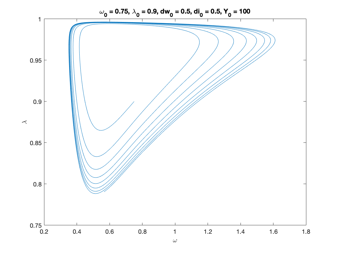
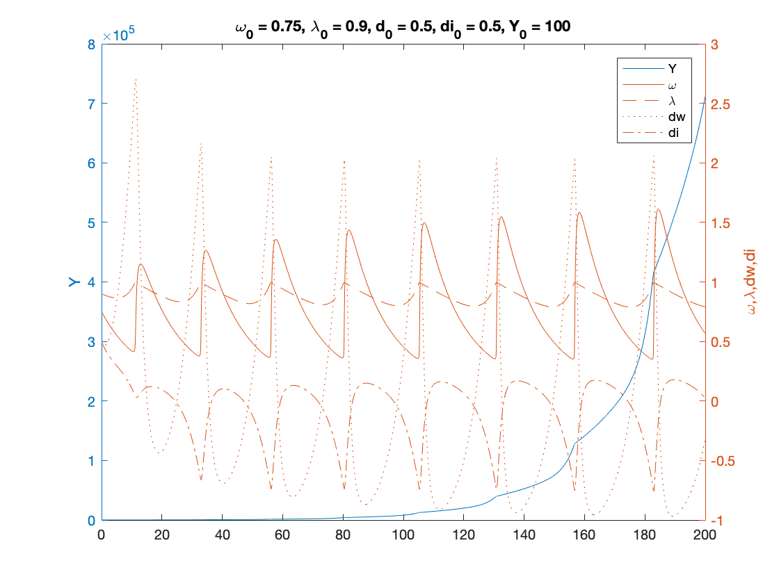
% Parameters as in Table 3 (modified for two classes), except for eta_p, gamma

nu = 3; %capital to output ratio
alpha = 0.025; %productivity growth rate
beta = 0.02; %population growth rate
delta = 0.05; %depreciation rate
r = 0.03; %real interest rate
eta_p = 0.5; % adjustment speed for prices - MODIFIED (this is 0.45 in the paper)
markup = 1.6; % mark-up value
gamma = 0.96; % (1-gamma) is the degree of money ilusion - MODIFIED
theta = 0.2; % proportion of profits paid to investors - MODIFIED
x=[];

phi0 = 0.04/(1-0.04^2); %Phillips curve parameter
phi1 = 0.04^3/(1-0.04^2); %Phillips curve parameter
 c_minus_w = 0.02; % consumption share hard-lower bound for workers - MODIFIED
 c_minus_i = 0.01; % consumption share hard-lower bound for investors - MODIFIED
 A_c = 0; %Consumption share asymptotic lower bound
 B_c = 8; % Consumption share growth rate (NOTE: this is 5 in the paper)
 C_c = 1;
 K_w = 0.75; % Consumption share upper bound for workers - MODIFIED
 K_i = 0.15; % Consumption share upper bound for investors - MODIFIED
 nu_c = 0.2;
 Q_w= ((K_w-A_c)/(c_minus_w-A_c))^nu_c-C_c;
 Q_i= ((K_i-A_c)/(c_minus_i-A_c))^nu_c-C_c;


fun_consumption_w =@(x) max(c_minus_w,A_c + ((K_w-A_c)./(C_c+Q_w*exp(-B_c*x)).^(1/nu_c))); %----first specification : generalised logistic consumption function------%
fun_consumption_w_inv = @(x) -log((((K_w-A_c)./(x-A_c)).^nu_c-C_c)./Q_w)./B_c; % inverse of the consumption function over positive income

fun_consumption_i =@(x) max(c_minus_i,A_c + ((K_i-A_c)./(C_c+Q_i*exp(-B_c*x)).^(1/nu_c))); %----first specification : generalised logistic consumption function------%
fun_consumption_i_inv = @(x) -log((((K_i-A_c)./(x-A_c)).^nu_c-C_c)./Q_i)./B_c; % inverse of the consumption function over positive income

total_consumption =@(x) fun_consumption_w(x)+fun_consumption_i(x);

% Numerical Values of Interest
c_eq=1-nu*(alpha+beta+delta)

w_0=((r-alpha-beta)/eta_p+1)/markup


% Sample paths of the dual Keen model


omega0 = 0.75;
lambda0 = 0.9;
dw0 = 0.5;
di0 = 0.5;
Y0 = 100;
T = 200;


[tK,yK] = ode15s(@(t,y) two_class_dual_keen(y), [0 T], convert([omega0, lambda0, dw0,di0]), options);
yK = retrieve(yK);
Y_output = Y0*yK(:,2)/lambda0.*exp((alpha+beta)*tK);

n=length(yK(:,3))

omega_bar = yK(n,1)
lambda_bar = yK(n,2)
dw_bar = yK(n,3)
di_bar = yK(n,4)


figure(3)
plot(yK(:,1), yK(:,2)), hold on;
%plot(bar_omega_K, bar_lambda_K, 'ro')
xlabel('\omega')
ylabel('\lambda')
title(['\omega_0 = ', num2str(omega0, txt_format), ...
    ', \lambda_0 = ', num2str(lambda0, txt_format), ...
    ', dw_0 = ', num2str(dw0, txt_format), ...
    ', di_0 = ', num2str(di0, txt_format), ...
    ', Y_0 = ', num2str(Y0, txt_format)])

print('two_keen_phase_cycle','-depsc')

figure(4)
yyaxis right
plot(tK, yK(:,1),tK,yK(:,2),tK,yK(:,3),tK,yK(:,4))
ylabel('\omega,\lambda,dw,di')

yyaxis left
plot(tK, Y_output)
ylabel('Y')


title(['\omega_0 = ', num2str(omega0,txt_format), ...
    ', \lambda_0 = ', num2str(lambda0, txt_format), ...
    ', d_0 = ', num2str(dw0, txt_format), ...
    ', di_0 = ', num2str(di0, txt_format), ...
    ', Y_0 = ', num2str(Y0, txt_format)])
legend('Y','\omega', '\lambda','dw','di')
print('two_keen_time_cycle','-depsc')
c_eq =

    0.7150


w_0 =

    0.6062


n =

        3228


omega_bar =

    0.5668


lambda_bar =

    0.7906


dw_bar =

   -0.3172


di_bar =

    0.0224
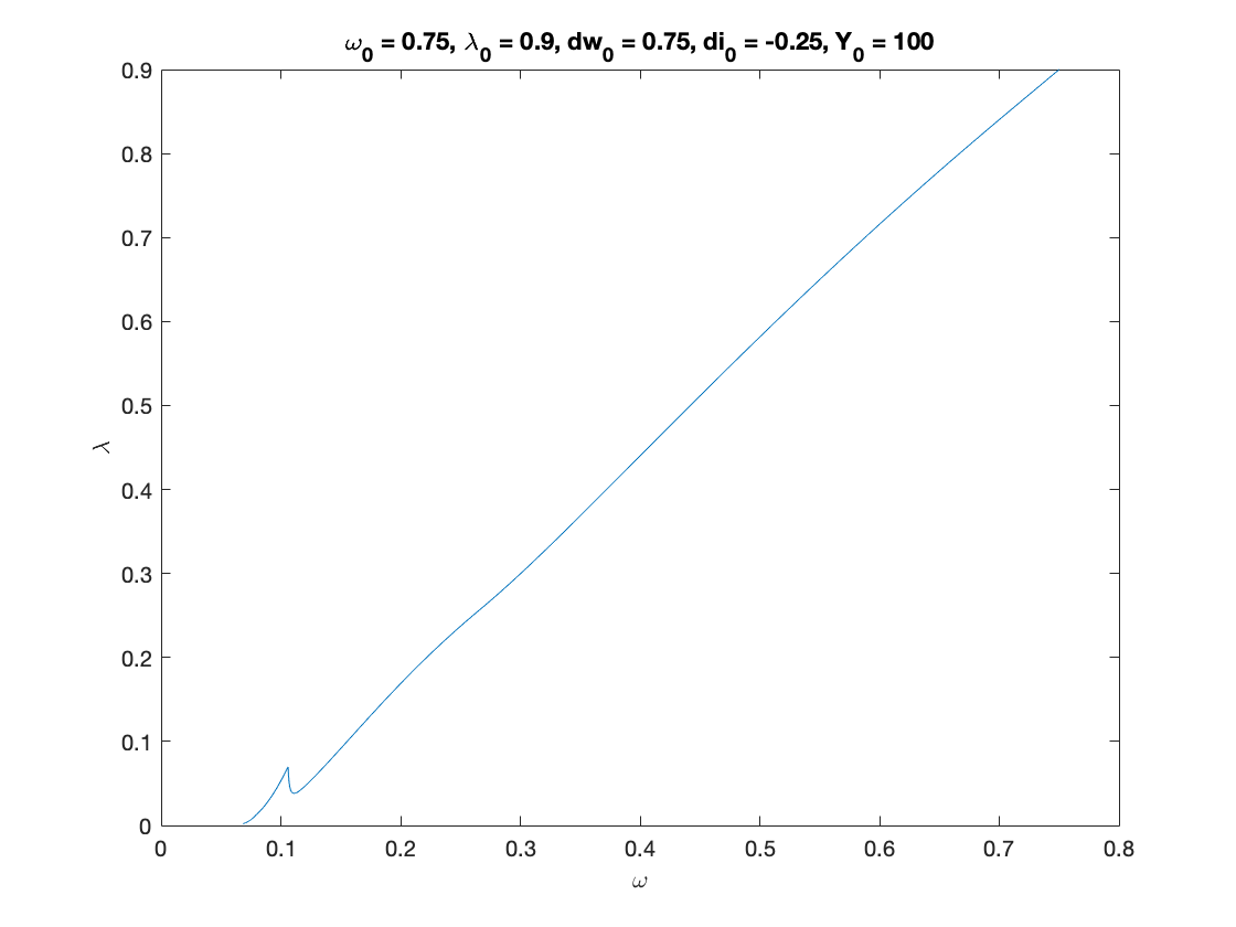
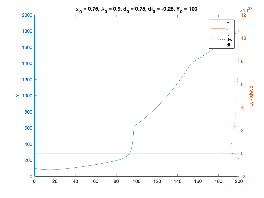
Example 3
% Parameters as in Table 3 (modified for two classes), except for nu

nu = 15; %capital to output ratio - MODIFIED
alpha = 0.025; %productivity growth rate
beta = 0.02; %population growth rate
delta = 0.05; %depreciation rate
r = 0.03; %real interest rate
eta_p = 0.35; % adjustment speed for prices
markup = 1.6; % mark-up value
gamma = 0.8; % (1-gamma) is the degree of money ilusion
theta = 0.2; % proportion of profits paid to investors - MODIFIED
x=[];

phi0 = 0.04/(1-0.04^2); %Phillips curve parameter
phi1 = 0.04^3/(1-0.04^2); %Phillips curve parameter
 c_minus_w = 0.02; % consumption share hard-lower bound for workers - MODIFIED
 c_minus_i = 0.01; % consumption share hard-lower bound for investors - MODIFIED
 A_c = 0; %Consumption share asymptotic lower bound
 B_c = 5; % Consumption share growth rate
 C_c = 1;
 K_w = 0.75; % Consumption share upper bound for workers - MODIFIED
 K_i = 0.15; % Consumption share upper bound for investors - MODIFIED
 nu_c = 0.2;
 Q_w= ((K_w-A_c)/(c_minus_w-A_c))^nu_c-C_c;
 Q_i= ((K_i-A_c)/(c_minus_i-A_c))^nu_c-C_c;


fun_consumption_w =@(x) max(c_minus_w,A_c + ((K_w-A_c)./(C_c+Q_w*exp(-B_c*x)).^(1/nu_c))); %----first specification : generalised logistic consumption function------%
fun_consumption_w_inv = @(x) -log((((K_w-A_c)./(x-A_c)).^nu_c-C_c)./Q_w)./B_c; % inverse of the consumption function over positive income

fun_consumption_i =@(x) max(c_minus_i,A_c + ((K_i-A_c)./(C_c+Q_i*exp(-B_c*x)).^(1/nu_c))); %----first specification : generalised logistic consumption function------%
fun_consumption_i_inv = @(x) -log((((K_i-A_c)./(x-A_c)).^nu_c-C_c)./Q_i)./B_c; % inverse of the consumption function over positive income

total_consumption =@(x) fun_consumption_w(x)+fun_consumption_i(x);

% Numerical Values of Interest
c_eq=1-nu*(alpha+beta+delta)

w_0=((r-alpha-beta)/eta_p+1)/markup


% Sample paths of the dual Keen model


omega0 = 0.75;
lambda0 = 0.9;
dw0 = 0.75;
di0 = -0.25;
Y0 = 100;
T = 200;


[tK,yK] = ode15s(@(t,y) two_class_dual_keen(y), [0 T], convert([omega0, lambda0, dw0,di0]), options);
yK = retrieve(yK);
Y_output = Y0*yK(:,2)/lambda0.*exp((alpha+beta)*tK);

n=length(yK(:,3))

omega_bar = yK(n,1)
lambda_bar = yK(n,2)
dw_bar = yK(n,3)
di_bar = yK(n,4)


figure(5)
plot(yK(:,1), yK(:,2)), hold on;
%plot(bar_omega_K, bar_lambda_K, 'ro')
xlabel('\omega')
ylabel('\lambda')
title(['\omega_0 = ', num2str(omega0, txt_format), ...
    ', \lambda_0 = ', num2str(lambda0, txt_format), ...
    ', dw_0 = ', num2str(dw0, txt_format), ...
    ', di_0 = ', num2str(di0, txt_format), ...
    ', Y_0 = ', num2str(Y0, txt_format)])

print('two_keen_phase_divergent','-depsc')

figure(6)
yyaxis right
plot(tK, yK(:,1),tK,yK(:,2),tK,yK(:,3),tK,yK(:,4))
ylabel('\omega,\lambda,dw,di')

yyaxis left
plot(tK, Y_output)
ylabel('Y')


title(['\omega_0 = ', num2str(omega0,txt_format), ...
    ', \lambda_0 = ', num2str(lambda0, txt_format), ...
    ', d_0 = ', num2str(dw0, txt_format), ...
    ', di_0 = ', num2str(di0, txt_format), ...
    ', Y_0 = ', num2str(Y0, txt_format)])
legend('Y','\omega', '\lambda','dw','di')
print('two_keen_time_divergent','-depsc')
c_eq =

   -0.4250


w_0 =

    0.5982


n =

   870


omega_bar =

    0.0683


lambda_bar =

    0.0020


dw_bar =

   1.0148e+24


di_bar =

  -5.6200e+22
Auxiliary functions
Instead of integrating the system in terms of omega, lambda and d, we decided to use:
log_omega = log(omega), tan_lambda = tan((lambda-0.5)*pi), and y_h=omega-r*d disposable income of households
Experiments show that the numerical methods work better with these variables.
function new = convert(old)
    % This function converts
    % [omega, lambda, d, p]
    % to
    % [log_omega, tan_lambda, y]
    % It also work with the first 2 components alone.
    % each of these variables might also be a time-dependent vector

    n = size(old,2); %number of variables
    new = zeros(size(old));

    new(:,1) = log(old(:,1));
    new(:,2) = tan((old(:,2)-0.5)*pi);
    if n>2
        new(:,3) = old(:,1)-r.*old(:,3);
        if n==4
            new(:,4) = theta*(1-old(:,1)+r*(old(:,3)+old(:,4))-delta*nu)-r*old(:,4);
        end
    end
end

function old = retrieve(new)
    % This function retrieves [omega, lambda, d, p]
    % from
    % [log_omega, tan_lambda, pi_n, log_p]
    %
    %  It also work with the first 2 or 3 elements alone.
    % each of these variables might also be a time-dependent vector

    n = size(new,2); %number of variables
    old = zeros(size(new));

    old(:,1) = exp(new(:,1));
    old(:,2) = atan(new(:,2))/pi+0.5;
    if n>2
        old(:,3) = (old(:,1)-new(:,3))./r;
        if n==4
            old(:,4) = (theta*(1-old(:,1)+r*old(:,3)-delta*nu)-new(:,4))/(r*(1-theta));
        end
    end
end


function f = two_class_dual_keen(y)
    f = zeros(4,1);
    log_omega = y(1);
    tan_lambda = y(2);
    y_w = y(3);
    y_i = y(4);
    lambda = atan(tan_lambda)/pi+0.5;
    omega = exp(log_omega);
    g_Y = (1-fun_consumption_w(y_w)-fun_consumption_i(y_i))./nu-delta;

    f(1) = fun_Phi(lambda)-alpha-(1-gamma)*eta_p*(markup*omega-1); %d(log_omega)/dt
    f(2) = (1+tan_lambda^2)*pi*lambda*(g_Y-alpha-beta); %d(tan_lambda)/dt
    f(3) = omega*f(1)-r*(fun_consumption_w(y_w)-y_w)+(omega-y_w)*(g_Y+eta_p*(markup*omega-1)); %d(y_w)/dt
    f(4) = -theta*omega*f(1)+theta*r*(fun_consumption_w(y_w)-y_w)-(1-theta)*r*(fun_consumption_i(y_i)-y_i)+(theta*(1-omega-delta*nu)-y_i)*(g_Y+eta_p*(markup*omega-1)); %d(y_i)/dt
end
end