The problem is simplified by assuming that all stays are exactly 1 day, so we only need to look at the cumulative probability distribution for X = the number of admissions, assuming a Poisson distribution with mean = 2.
> ppois(0:7,2)
[1] 0.1353353 0.4060058 0.6766764 0.8571235 0.9473470 0.9834364 0.9954662
[8] 0.9989033
So we could either say that 4 beds will be enough since P[X <= 4] = 0.95, or we could look at the numbers to more than 2 decimal places and claim that 5 beds are required to ensure that the probability is at least 95%. Note that we could have solved directly with the Poisson quantile function:
> qpois(.95,2)
[1] 5
Similarly, on high pollution days when the mean number of admissions is 4 per day, either 7 or 8 beds is an acceptable answer.
> ppois(5:10,4)
[1] 0.7851304 0.8893260 0.9488664 0.9786366 0.9918678 0.9971602
> qpois(.95,4)
[1] 8
Using Total Probability, P[X = 4] = P[X = 4 | normal pollution] P[normal pollution] + P[X = 4 | high pollution] P[high pollution]
> dpois(4,2)*(345/365) + dpois(4,4)*(20/365)
[1] 0.0959848
There are 41 twin pairs; to show the lumbar spine differences and count the number of negative differences, use
> ls2-ls1
 [1] -0.05 -0.12 -0.24  0.04 -0.19 -0.03 -0.08 -0.10  0.15 -0.12 -0.10  0.09
[13] -0.08 -0.07 -0.03  0.05  0.04 -0.04 -0.01 -0.06 -0.11 -0.05  0.03 -0.12
[25]  0.03  0.01  0.07  0.13 -0.03 -0.21 -0.05  0.03 -0.05 -0.01  0.11 -0.07
[37] -0.08 -0.08 -0.07  0.10 -0.10
> length(ls2)
[1] 41
> sum(ls2-ls1<0)
[1] 28
If there were no difference between the heavier smoking twin and the lighter smoking twin, the number of negative differences would be Bin(41, 0.5), in which case the probability of getting 28 or more negative differences would be
> 1-pbinom(27,41,0.5)
[1] 0.01376658
which is less than 5%. Since what was observed would be unlikely under the hypothesis, there is evidence from the data that the heavier smoking twin tends to have the lighter lumbar spine bone density.
We can order the twins in ascending order according to their pack-year differences, then take lumbar spine differences of the 20 twins with the highest pack-year differences and find that 17 of the 20 lumbar spine differences are negative.
> sum((ls2-ls1)[order(pyr2-pyr1)][22:41]<0)
[1] 17
> 1-pbinom(16,20,0.5)
[1] 0.001288414
The probability of getting 17 or more negative lumber spine differences out of 20 under the hypothesis of indifference is even smaller when we consider only the twins with the biggest pack-year differences.
> ncases <- c(13, 8, 13, 13, 9, 10, 8, 8, 11, 5)
> mean(ncases)
[1] 9.8
> ncpw <- 7*mean(ncases)/365
> ncpw
[1] 0.1879452
> dpois(0, 6*ncpw)
[1] 0.3237864
> dpois(0, 6*ncpw)*(1-dpois(0, ncpw))
[1] 0.05547753
Let Xt be the number of cases in a t-week period. Scaling the mean number of cases per year gives a mean number of 0.188 cases per week; I have based the conversion on a 365-day year, you will get a slightly different value if you assume a 52-week year. (a) P[X6 = 0] = 0.324; (b) since non-overlapping intervals are independent in a Poisson process, past history is not relevant and the answer is the same as in (a); since the next 6 weeks are independent of the 7th week and we need the probability of no cases in the next 6 weeks then at least one case in the 7th week, P[X6 = 0]P[X1 > 0] = P[X6 = 0]{1-P[X1 = 0]} = 0.0555.
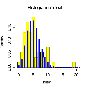
> mean(nleaf)
[1] 5.056604
> var(nleaf)
[1] 11.47750
> var(nleaf)/mean(nleaf)
[1] 2.269805
> hist(nleaf,breaks=seq(-.5,20.5,by=1),prob=T,col="yellow")
> lines(0:21,dpois(0:21,mean(nleaf)),lwd=3,type="h",col="blue")
There is evidence of overdispersion: the ratio of variance to mean is 2.27 which is >> 1, and the histogram shows more probability in the left and right tails and less in the centre, compared to the Poisson distribution.
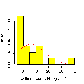
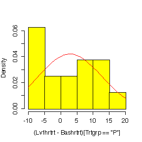
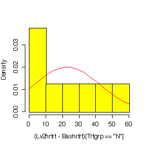
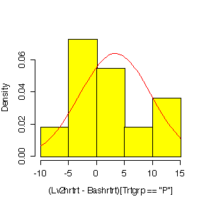
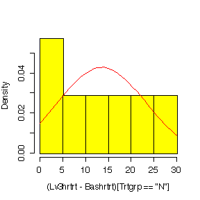
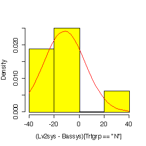
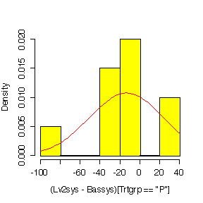
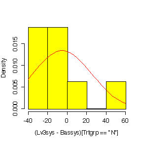
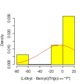
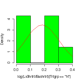
Here is the code for one of the graphs, plotting on the original scale:
> hist((Lv3hrtrt-Bashrtrt)[Trtgrp=="N"],prob=T,col="yellow")
> diff <- (Lv3hrtrt-Bashrtrt)[Trtgrp=="N"]
> xgr <- seq(0,30,len=40)
> lines(xgr,dnorm(xgr,mean(diff,na.rm=T),sqrt(var(diff,na.rm=T))),col="red")
|
|
|
|
|
|
|
|
|
|
|
|
|
|
|
|
|
|
|
|
|
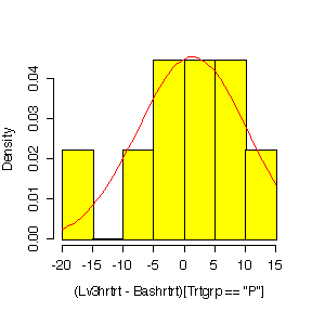
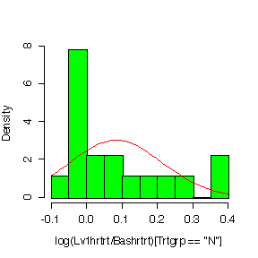
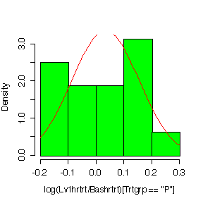
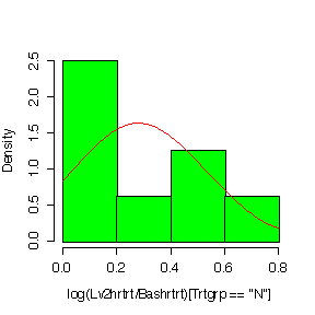
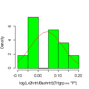
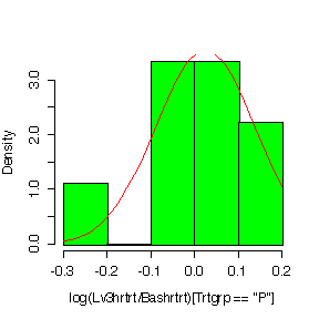
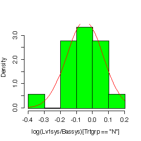
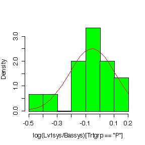
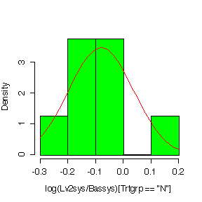
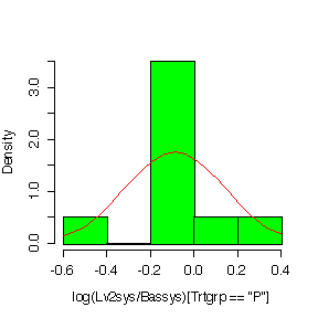
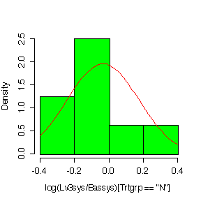
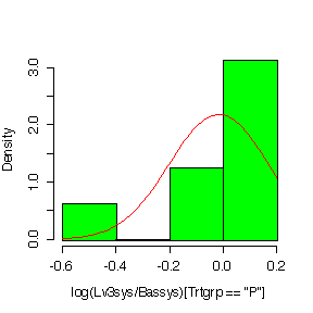
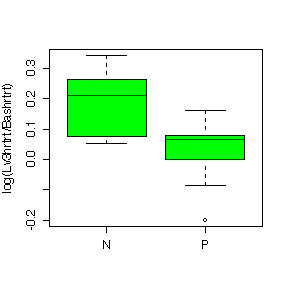
Plotting on a log scale:
> hist(log(Lv3sys/Bassys)[Trtgrp=="P"],prob=T,col="green")
> diff<-log(Lv3sys/Bassys)[Trtgrp=="P"]
> xgr<-seq(-.6,.2,len=40)
> lines(xgr,dnorm(xgr,mean(diff,na.rm=T),sqrt(var(diff,na.rm=T))),col="red")
It is hard to judge normality with such small samples, but in most cases the histograms on the log scale look a bit more symmetric than the histograms in the original units.
|
|
|
|
|
|
|
|
|
|
|
|
|
|
|
|
|
|
|
|
|
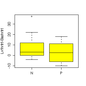
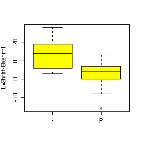
Here is the code for the first box plot:
> boxplot(split(Lv1hrtrt-Bashrtrt,Trtgrp),ylab="Lv1hrtrt-Bashrtrt",col="yellow")
|
|
|
|
|
|
|
|
|
|
|
|
|
|
|
|
|
|
|
|
|
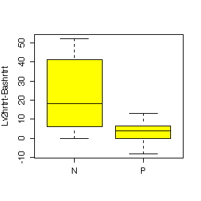
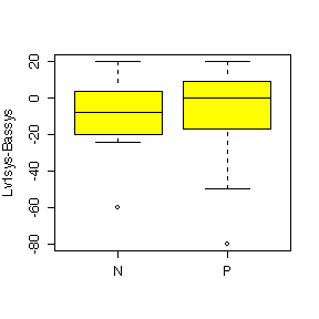
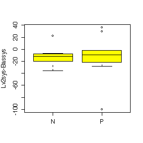
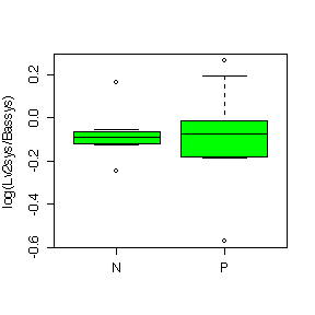
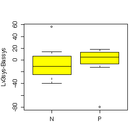
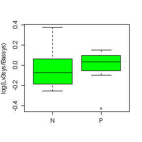
The difference between Nifedipine and Propanolol is more evident for heart rate than for systolic blood pressure. Nifedipine generally raises heart rate above the baseline level; the effect is similar to Propanolol at Level 1 but Nifedipine gives a huger median effect than Propanolol at Level 2 and Level 3; it gives a much more variable effect than Propanolol at Level 2. Nipfedipine is seen to lower systolic blood pressure at Level 3 but is not much different from Propanolol at Levels 1 and 2.
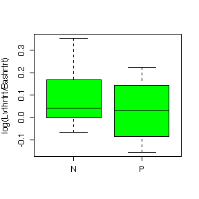
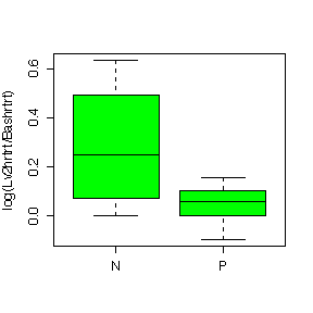
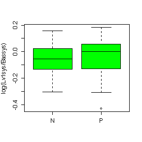
The box plots in log units are very similar to the box plots in original units so the choice of units does not affect our interpretation of the data.
Let X be the total weight of 10 people in kg. Assuming independence of the people, E[X] = 10*65 and Var[X] = 10*81; assuming that the sum is approximately normal (and the Central Limit Theorem guarantees that the sum will be closer to normal than the distribution of the weight of an individual), P[X > 700] = F((700-650)/sqrt(810)) = 0.03947.
Let Y be the number of loads out of 5 that exceed 700; assuming independence of the loads, Y ~ Bin(5, P[X>700]) so P[Y<=1] = 0.9856.
> pr <- 1-pnorm(700,10*65,sqrt(10*81))
> pr
[1] 0.03947417
> pbinom(1,5,pr)
[1] 0.985612
The p.d.f. for the U(-0.5, 0.5) distribution is f(x) = 1 when -0.5 < x < 0.5 and 0 otherwise. Integrating x dx from -0.5 to 0.5 gives that E[X] = 0 (which was obvious from symmetry) and integrating x^2 dx from -0.5 to 0.5 gives that Var[X] = 1/12; i.e.
Hence the sum of 12 U(-0.5, 0.5) random variables has mean 0 and variance 12*(1/12) = 1 and is approximately normal by the Central Limit Theorem, so we have that X1 + ... + X12 ~ AN(0, 1) where the approximation to normality is in fact very good.
You can change a U(0, 1) variate to a U(-0.5, 0.5) variate by subtracting 0.5, so you can generate N(0, 1) random variables on your calculator by adding up 12 U(0, 1) random numbers and subtracting 6. I repeated this 5 times on my calculator and got the following random numbers:
-0.0697849 0.9950637 -1.1663607 -1.1704401 -1.2009249
Derivation of the formula is a straightforward application of either Equation 5.13 on page 138 or its matrix version and will not be given here.
Note that the variance of the sample mean increases from s2/n (the well-known formula for independent identically distributed observations) when r = 0, to 3 s2/n when r = 1 and n is large.
This illustrates how positive autocorrelation in repeated laboratory measurements increases the standard error (and hence decreases the precision) of the sample mean.
A negative r will reduce the variance of the sample mean, as the data will tend to lie more evenly on either side of the mean than independent data, but note that there are restrictions; for example, since the variance of the sample mean can't be negative, we can only have r > -n/(2*(n-1)).
Give n = 200, xbar = 140, s = 25, the 95% confidence interval for the true mean systolic blood pressure is given by
> 140 + c(-1, 1)*qnorm(0.975)*25/sqrt(200)
[1] 136.5352 143.4648
Since the population average for people of comparable age is 130 mm Hg and this lies below the 95% confidence interval, there is evidence at the 95% level of confidence that people with glaucoma have a higher systolic blood pressure than people of comparable age without glaucoma.
Here are the calculations, statistics and confidence intervals for the four cases requested. Note that we have to be careful to eliminate missing values from all calculations. The comparative box plots were given in the answer to 5.56 and need not be repeated here.
Note that all of the confidence intervals include 0 except Heart Rate with Nifedipine. Hence, with that exception, there is no evidence of a treatment effect at Level 1.
Heart Rate - Nifedipine
> diff <- (Lv1hrtrt-Bashrtrt)[Trtgrp=="N"]
> n <- sum(!is.na(diff))
> xbar <- mean(diff,na.rm=T)
> s <- sqrt(var(diff,na.rm=T))
> c(n=n,xbar=xbar,s=s)
        n      xbar         s
18.000000  6.111111 10.665441
> xbar + c(-1,1)*qt(.975,n-1)*s/sqrt(n)
[1]  0.807312 11.414910
Heart Rate - Propanolol
> diff <- (Lv1hrtrt-Bashrtrt)[Trtgrp=="P"]
> n <- sum(!is.na(diff))
> xbar <- mean(diff,na.rm=T)
> s <- sqrt(var(diff,na.rm=T))
> c(n=n,xbar=xbar,s=s)
        n      xbar         s
16.000000  2.875000  9.457801
> xbar + c(-1,1)*qt(.975,n-1)*s/sqrt(n)
[1] -2.164706  7.914706
Systolic Blood Pressure - Nifedipine
> diff <- (Lv1sys-Bassys)[Trtgrp=="N"]
> n <- sum(!is.na(diff))
> xbar <- mean(diff,na.rm=T)
> s <- sqrt(var(diff,na.rm=T))
> c(n=n,xbar=xbar,s=s)
        n      xbar         s
18.000000 -7.944444 18.694045
> xbar + c(-1,1)*qt(.975,n-1)*s/sqrt(n)
[1] -17.240774   1.351885
Systolic Blood Pressure - Propanolol
> diff <- (Lv1sys-Bassys)[Trtgrp=="P"]
> n <- sum(!is.na(diff))
> xbar <- mean(diff,na.rm=T)
> s <- sqrt(var(diff,na.rm=T))
> c(n=n,xbar=xbar,s=s)
        n      xbar         s
15.000000 -8.933333 26.606838
> xbar + c(-1,1)*qt(.975,n-1)*s/sqrt(n)
[1] -23.667709   5.801042
Here there are complete data on 41 twin pairs with no missing values, so the calculation of the confidence intervals can be done more simply.
Femoral Neck
> mean(fn2-fn1) + c(-1,1)*qt(.975,40)*sqrt(var(fn2-fn1)/41)
[1] -0.03012505  0.02866164
Femoral Shaft
> mean(fs2-fs1) + c(-1,1)*qt(.975,40)*sqrt(var(fs2-fs1)/41)
[1] -0.066703514  0.005727904
In both cases the 95% confidence interval includes 0 so there is no evidence from these data, at the 95% level of confidence, that bone density in the femoral neck or the femoral shaft is associated with number of pack years smoked.