[Full marks = 140]
Suppose you want to find a two-sided 99% confidence interval for the variance of a normal population. How many observations are needed to ensure that the upper limit is no more than 4 times the lower limit? Will this calculation be valid for non-normal data?
Since the upper limit divided by the lower limit is just the ratio of the 99.5% quantile over the 0.5% quantile, we can try different degrees of freedom and see that the ratio is less than 4 for 29 degrees of freedom; since df = n - 1, this means that 30 observations are needed.
> qchisq(.995,27:30)/qchisq(.005,27:30)
[1] 4.204493 4.092128 3.988646 3.893019
Since the sample variance follows a chi-square distribution only if samples are from a normal distribution, this calculation will not be valid for non-normal data. (Specifically, it will be too narrow if the samples come from a distribution with heavier tails than the normal, and too wide if the samples come from a distribution with lighter tails than the normal.)
If your time to run a marathon has a mean of 4 hr 10 min with a standard deviation of 15 min, and your friend's time has a mean of 3 hr 55 min with a standard deviation of 10 min, and you both run in the same race, what is the probability that you will finish ahead of your friend? State any assumptions you make and discuss their validity in this example.
Let X be your time and Y your friend's time; we need to calculate P[X - Y < 0]. Now, E[X - Y] = E[X] - E[Y] = 15 min and assuming independence Var[X - Y] = Var[X] + Var[Y] = 152 + 102 = 325, hence assuming normality of X - Y, P[X - Y <0] = F((0 -15)/sqrt(325)) = 0.203
> pnorm((0-15)/sqrt(325))
[1] 0.2026903
The independence assumption is probably invalid if you can see each other and run together for any part of the race.
The normality assumption might be OK; you would need to look at some data to test it but I can't see how you could get a large sample of marathon times from the same person. At least X - Y will be more normal than either X or Y alone.
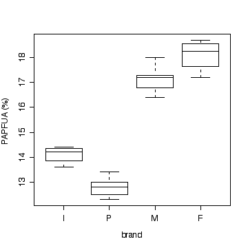
Samples of four different brands of diet margarine were analysed to determine the percentage of physiologically active polyunsaturated fatty acids (PAPFUA). Give an appropriate analysis, including an ANOVA table and a graph. Give a 95% confidence interval for the residual variance. State any assumptions you make and do what you can to test the assumptions. State your conclusions.
Brand           PAPFUA (%)
Imperial:       14.1  13.6  14.4  14.3
Parkay:         12.8  12.5  13.4  13.0  12.3
Mazola:         16.8  17.2  16.4  17.3  18.0
Fleischmann's:  18.1  17.2  18.7  18.4
> marg
   poly brand
1  14.1     I
2  13.6     I
3  14.4     I
4  14.3     I
5  12.8     P
6  12.5     P
7  13.4     P
8  13.0     P
9  12.3     P
10 16.8     M
11 17.2     M
12 16.4     M
13 17.3     M
14 18.0     M
15 18.1     F
16 17.2     F
17 18.7     F
18 18.4     F

> boxplot(split(marg$poly,marg$brand)[c("I","P","M","F")],xlab="brand",ylab="PAPFUA (%)")

Note that a multiple dot plot would also be acceptable.
> anova(lm(poly~brand, data=marg))
Analysis of Variance Table

Response: poly
          Df Sum Sq Mean Sq F value    Pr(>F)
brand      3 84.764  28.255  103.77 8.428e-10 ***
Residuals 14  3.812   0.272
---
Signif. codes:  0 `***' 0.001 `**' 0.01 `*' 0.05 `.' 0.1 ` ' 1
The following code extracts the residual mean squared error from the anova table and uses it to compute the chi-squared confidence limits on 14 degrees of freedom for residual variance as (0.146, 0.677).
> anova(lm(poly~brand, data=marg))$"Mean Sq"[2]

0.2722857

> anova(lm(poly~brand, data=marg))$"Mean Sq"[2]/c(qchisq(.975,14)/14,qchisq(.025,14)/14)
[1] 0.1459477 0.6772403
There is strong evidence (P << 0.001) that the percentage of physiologically active polyunsaturated fatty acids varies between these four brands of margarine.
(a) Two types of fish attractors, one made from clay pipes and the other from cement blocks and brush, were used over 8 consecutive time periods spanning two years at Lake Tohopekaliga, Florida. The data give fish caught per fishing day in each time period.
period    1    2    3    4    5    6    7    8
pipe   6.64 7.89 1.83 0.42 0.85 0.29 0.57 0.63
brush  9.73 8.21 2.17 0.75 1.61 0.75 0.83 0.56
Is there evidence that one attractor is more effective than the other? Which is the most appropriate analysis: a two-sample t-test, a paired t-test, or a paired t-test on log-transformed data? Give a p-value. State your assumptions and your conclusions.
The paired t-test on log-transformed data would be best because the spread is greater at the higher catches and the difference in logs (or log of ratios) is less skewed than the distribution of differences on the original scale.The paired t-test would be OK, the two-sample t-test would be inappropriate.
|
|
|
|
|
|
|
|
|
The differences (on original or log scales) are assumed to be independent (suspect because these are consecutive periods) and normal. The sample is too small to test either assumption, but the dot plots and the histograms suggest that differences on the log scale are more normal than differences in original units.
The t-test of the differences is not significant (P = 0.09), the t-test on the log ratios is significant (P = 0.02), but the t-test on log ratios is more valid, so there is evidence of a difference between the two attractors.
> fish$brush-fish$pipe
[1]  3.09  0.32  0.34  0.33  0.76  0.46  0.26 -0.07
> mean(fish$brush-fish$pipe)
[1] 0.68625
> var(fish$brush-fish$pipe)
[1] 0.9955982

> t.test(fish$brush,fish$pipe,pair=T) [4]
	 Paired t-test

data:  fish$brush and fish$pipe
t = 1.9453, df = 7, p-value = 0.0928
alternative hypothesis: true difference in means is not equal to 0
95 percent confidence interval:
 -0.1479289  1.5204289
sample estimates:
mean of the differences
                0.68625

> log(fish$brush)-log(fish$pipe)
[1]  0.38210193  0.03975679  0.17041120  0.57981850
[5]  0.63875311  0.95019228  0.37578934 -0.11778304
> mean(log(fish$brush)-log(fish$pipe))
[1] 0.37738
> var(log(fish$brush)-log(fish$pipe))
[1] 0.1199211

> t.test(log(fish$brush),log(fish$pipe),pair=T)

	 Paired t-test

data:  log(fish$brush) and log(fish$pipe)
t = 3.0823, df = 7, p-value = 0.01776
alternative hypothesis: true difference in means is not equal to 0
95 percent confidence interval:
 0.08786906 0.66689097
sample estimates:
mean of the differences
                0.37738
(b) Answer (a) using the sign test. State your assumptions and your conclusions.
Since 7 out of the 8 differences are positive, the P-value for the 2-sided sign test is
> 2*(1-pbinom(6,8,.5))
[1] 0.0703125
or by the normal approximation to the binomial with continuity correction
> 2*(1-pnorm((7-8/2-.5)/sqrt(8/4)))
[1] 0.07709987
so there is no evidence of a difference between the two attractors.
This test assumes only independence; but this assumption is suspect because the time periods are consecutive.
(c) Suppose that you are planning a larger study of the same attractors in the same lake. If one attractor attracts 50% more fish than the other, how many time periods would you need to ensure that a 5% test has a power of 99%?
Use Eqn 7.28 on page 241 of Rosner. Even though we are testing a mean difference, it is still a one-sample test. If one attractor attracts 50% more fish than the other, on the log scale we have D1 = log(1.5m) - log(m) = log(1.5). From (b), for the log-transformed data, s2 = 0.120. Hence the required number of periods will be 14.
> qnorm(0.99)
[1] 2.326348
> qnorm(0.975)
[1] 1.959964
> var(log(fish$brush)-log(fish$pipe))*((qnorm(0.99)+qnorm(0.975))/log(1.5))^2
[1] 13.40159
If we keep to the original units, D1 = (1.5m - m) = 0.5 m. We can estimate m by the mean of the pipe values (the smaller of the two means) and s2 by the sample variance of the differences, which is s2 = 0.996, so the required number of periods will be 13.
> var(fish$brush-fish$pipe)*((qnorm(0.99)+qnorm(0.975))/(0.5*mean(fish$pipe)))^2
[1] 12.80902
A camera was developed to determine the gray level over the lens of the human eye. Twelve patients were randomly selected, six with normal eyes and another six with cataractous eyes. One eye was tested on each patient. The data show the gray level on a scale of 1 (black) to 256 (white).
patient        1   2   3   4   5   6
cataractous  161 140 136 171 106 149
normal       158 182 185 145 167 177
(a) Display the data on an appropriate graph. Is there evidence of a significant difference between the two groups? Give a p-value, state your assumptions and your conclusions, and do what you can to assess the validity of your assumptions.
> t.test(eyecat, eyenor, var.equal = T)

	  Two Sample t-test

data:  eyecat and eyenor
t = -2.2489, df = 10, p-value = 0.04827
alternative hypothesis: true difference in means is not equal to 0
95 percent confidence interval:
 -50.1007029  -0.2326304
sample estimates:
mean of x mean of y
 143.8333  169.0000

> sqrt(var(eyecat))
[1] 22.65760
> sqrt(var(eyenor))
[1] 15.42725
> sqrt((5*var(eyecat)+5*var(eyenor))/10)
[1] 19.38255

> anova(lm(gray~cataract, data=eyes))
Analysis of Variance Table

Response: gray
          Df Sum Sq Mean Sq F value  Pr(>F)
cataract   1 1900.1  1900.1  5.0577 0.04827 *
Residuals 10 3756.8   375.7
---
Signif. codes:  0  `***'  0.001  `**'  0.01  `*'  0.05  `.'  0.1  ` '  1
Independence within and between samples (can't test); Normality (samples too small to test but looks OK on plot); Homoscdedasticity (looks OK on box plot, not rejected by F-test below, P = 0.42).
> F0 <- var(eyecat)/var(eyenor)
> F0
[1] 2.157003
> 2*(1-pf(F0,5,5))
[1] 0.4187581
Some evidence (P = 0.048) of a difference in mean gray level between normal and cataractous eyes.
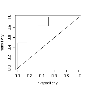
(b) How useful would this be as a screening test for cataracts? Plot a ROC curve. Choose a suitable cutoff. At this cutoff, what would the predictive value positive be if the prevalence of cataracts were 12% in the population being screened?
> sort(eyecat)
[1] 106 136 140 149 161 171
> sort(eyenor)
[1] 145 158 167 177 182 185
Given: Prevalence = 0.12, low gray scale values indicate the condition.
Cutoff at 138 gives:
sens = 2/6, spec = 6/6, PV+ = 1, PV- = 0.917.
Cutoff at 142.5 gives:
sens = 3/6, spec = 6/6, PV+ = 1, PV- = 0.936.
Cutoff at 147 gives:
sens = 3/6, spec = 5/6, PV+ = 0.290, PV- = 0.924.
Cutoff at (143.8333 + 169)/2 = 156.4 gives:
sens = 4/6, spec = 5/6, PV+ = 0.353, PV- = 0.948.
Cutoff at 164 gives:
sens = 5/6, spec = 4/6, PV+ = 0.254, PV- = 0.967.
The best cutoff is between 140 and 145; a higher cutoff gives a much lower PV+ in return for a slightly higher PV-, a lower cutoff gives PV+ = 1 but with a slightly lower PV-.

Despite the low sensitivity, the test is useful for screening because it gives a high PV+ and a high PV-.
The following data are from a 1979 paper classifying 445 college students according to their level of marijuana use, and their parents' use of alcohol and psychoactive drugs. Do the data suggest that parental usage and student usage are independent in the population from which the sample was drawn? State your assumptions and your conclusions.
                        Student level of marijuana use
                          never  occasional  regular
Parental         neither    141          54       40
use of alcohol   one         68          44       51
& drugs          both        17          11       19
This is a 3 by 3 contingency table. If you enter it into a matrix, you can use the chisq.test() function.
(To help see that it is not a two-way ANOVA problem, note that the number of observations is 445, not 9. The table gives counts in the 9 categories of the cross-classification.)
> drugs <- matrix(c(141,68,17,54,44,11,40,51,19),nrow=3,dimnames=list(c("neither","one","both"),c("never","occasional","regular")))
> drugs
        never occasional regular
neither   141         54      40
one        68         44      51
both       17         11      19

> sum(drugs)
[1] 445
> apply(drugs,1,sum)
neither     one    both
    235     163      47
> apply(drugs,2,sum)
     never occasional    regular
       226        109        110

> chisq.test(drugs)

	Pearson's Chi-squared test

data:  drugs
X-squared = 22.3731, df = 4, p-value = 0.0001689

> chisq.test(drugs)$observed
        never occasional regular
neither   141         54      40
one        68         44      51
both       17         11      19
> chisq.test(drugs)$expected
            never occasional  regular
neither 119.34831   57.56180 58.08989
one      82.78202   39.92584 40.29213
both     23.86966   11.51236 11.61798
Subjects chosen independently of each other; students chosen independently of their parents' use of alcohol and drugs; expected counts large enough that the chi-squared distribution is a good approximation.
There is strong evidence (P < 0.001) from these data that students' use of marijuana is related to their parents' use of alcohol and drugs; in particular, if the parents used neither alcohol nor drugs, it is less likely that the student will use marijuana.
Analyze the following data from a study to determine the effect of different plate materials and ambient temperature on the effective life (in hours) of a storage battery. There were 3 replicates at each combination of material and temperature. Give a 99% confidence interval for the residual variance. State your assumptions and your conclusions.
                               Ambient temperature
                              low           medium             high
Plate material  1   130,  74, 155     34,  80,  40     20,  82,  70
                2   150, 159, 188    136, 106, 122     25,  58,  70
This is a two-way ANOVA problem; it is a 2 by 3 factorial design with 3 replications at each combination of plate material and ambient temperature, for a total of 18 observations. When you create the data frame, make sure that material is entered as a factor.
> battery
   life material   temp
1   130        1    low
2    74        1    low
3   155        1    low
4    34        1 medium
5    80        1 medium
6    40        1 medium
7    20        1   high
8    82        1   high
9    70        1   high
10  150        2    low
11  159        2    low
12  188        2    low
13  136        2 medium
14  106        2 medium
15  122        2 medium
16   25        2   high
17   58        2   high
18   70        2   high
> is.factor(battery$material)
[1] TRUE

> anova(lm(life~material*temp, data=battery))
Analysis of Variance Table

Response: life
              Df  Sum Sq Mean Sq F value    Pr(>F)
material       1  6013.4  6013.4  7.8612 0.0159320 *
temp           2 24080.8 12040.4 15.7402 0.0004419 ***
material:temp  2  4570.8  2285.4  2.9877 0.0885176 .
Residuals     12  9179.3   764.9
---
Signif. codes:  0  `***'  0.001  `**'  0.01  `*'  0.05  `.'  0.1  ` '  1

> mse <- anova(lm(life~material*temp, data=battery))$"Mean Sq"[4]
> mse
 764.9444
> qchisq(.995,12)
[1] 28.29952
> qchisq(.005,12)
[1] 3.073824
> c(mse/(qchisq(.995,12)/12), mse/(qchisq(.005,12)/12))
 324.3636 2986.2915
The 99% confidence interval for the residual variance is (324, 2986).
Note the c(2,3,1) in the code; that is because the temperature levels are by default in alphabetical order "high", "low", "medium" but I want them to appear in the order "low", "medium", "high" on the graphs.
> matplot(matrix(sapply(split(battery$life,battery$material:battery$temp),mean),ncol=2)[c(2,3,1),],type="l",xlab="Ambient temperature",ylab="Life")
> legend(2.2,160,lty=1:2,col=1:2,legend=c("Plate 1","Plate 2"))
> matplot(matrix(sapply(split(battery$life,battery$temp:battery$material),mean),ncol=3)[,c(2,3,1)],type="l",xlab="Plate material",ylab="Life")
> legend(1,160,lty=1:3,col=1:3,legend=c("low temp","medium temp","high temp"))
|
|
|
Independence, normality, homoscedasticity.
If we look only at the ANOVA table, the interaction between plate material and temperature is not significant (P = 0.09), so we can test main effects. The difference between temperatures is very highly significant and the difference between plate materials is significant. Hence we conclude that both the ambient temperature and the plate material affect mean battery life, and the difference between plate materials is the same at each ambient temperature.
Th intraction plots show the story in more detail. They suggest that there is no interaction between plate material and ambient temperature at low and medium temperatures (the lines are parallel and Plate material 2 gives a longer mean life than Plate material 1) but at high tempertures the mean life is much reduced and is about the same for both plate materials. The interaction is not, however, significant, so if high-temperature performance is important, further study and more data will be needed.
A study of nitrogen emissions from power boilers reported x = burner area liberation rate (in Mbtu/hr-ft2) and y = NOx emission rate (in ppm) for 14 boilers.
x 100  125  125  150  150  200  200  250  250  300  300  350  400  400
y 150  140  180  210  190  320  280  400  430  440  390  600  610  670
(a) Fit a straight line to the data by least squares, with NOx emission rate as the dependent variable. Plot the data and the fitted line on a graph. Can NOx emission rate be predicted as a linear function of burner area liberation rate? Present your analysis in an ANOVA table with F-Tests for non-linearity and for the slope of the regression line. Give a 95% confidence interval for the residual variance. State your assumptions and your conclusions.
> emission
     y   x
1  150 100
2  140 125
3  180 125
4  210 150
5  190 150
6  320 200
7  280 200
8  400 250
9  430 250
10 440 300
11 390 300
12 600 350
13 610 400
14 670 400
> plot(emission$x,emission$y)
> fitemission <- lm(y~x, data=emission)
> abline(fitemission)
> coef(fitemission)
(Intercept)           x
 -45.551905    1.711432
> anova(lm(y~x+as.factor(x), data=emission))
Analysis of Variance Table

Response: y
             Df Sum Sq Mean Sq  F value    Pr(>F)
x             1 398030  398030 450.6003 7.126e-07 ***
as.factor(x)  6  10905    1818   2.0576    0.2007
Residuals     6   5300     883
---
Signif. codes:  0 `***' 0.001 `**' 0.01 `*' 0.05 `.' 0.1 ` ' 1
Nonlinearity is not significant (P = 0.20), and the slope is very highly significant (P = 0.000001), so for the range of burner area liberation rates studied the emission rate can be predicted as a linear function of burner area liberation rate.
Independence, normality and homoscedasticity.
The MSE = 883.3 gives an estimate of residual variance on 6 degrees of freedom; the 95% confidence interval is (366.8, 4283).
> mse <- anova(lm(y~x+as.factor(x), data=emission))$"Mean Sq"[[3]]
> mse
[1] 883.3333
> mse/c(qchisq(0.975,6)/6, qchisq(0.025,6)/6)
[1]  366.7979 4283.3674
Since the lack of fit is not significant, we could also get the residual variance estimate from the regression ANOVA, this time on 12 degrees of freedom; the 95% confidence interval is (694.4, 3680).
> anova(lm(y~x, data=emission))
Analysis of Variance Table

Response: y
          Df Sum Sq Mean Sq F value    Pr(>F)
x          1 398030  398030  294.74 8.226e-10 ***
Residuals 12  16205    1350
---
Signif. codes:  0 `***' 0.001 `**' 0.01 `*' 0.05 `.' 0.1 ` ' 1

> mse <- anova(lm(y~x, data=emission))$"Mean Sq"[[2]]
> mse
[1] 1350.454
> mse/c(qchisq(0.975,12)/12, qchisq(0.025,12)/12)
[1]  694.4203 3679.8891
(b) Predict the NOx emission rate at burner area liberation rates 10 and 325. How reliable do you think your predictions are?
Since R2 = 0.96 is high, the points lie very close to a straight line and a linear predictor will be reliable, at least for interpolation.
The prediction of at x = 325 is valid because it is a linear interpolation.
The prediction at x = 10 is an extrapolation. Since the emission rate can't be negative, this prediction should not be considered reliable. [3]
> predict(lm(y~x, data=emission),data.frame(x=c(10,325)))
        1         2
-28.43758 510.66360
(a) In a genetics study, you plan to observe 20 F1 offspring. Your theory says that the probability of getting a wild-eyed female is 1/4 but you are concerned that the actual probability may be greater than 1/4. Using the exact binomial distribution, find a critical region such that the type I error rate is as close as possible to 5%. What is the exact significance level of the test? What is the probability of a type II error if the true probability of a wild-eyed female is 1/2? If the true probability of a wild-eyed female is 3/4?
The test statistic is the number of wild-eyed females; under the null hypothesis the reference distribution is Bin(20, 0.25). The alternative hypothesis suggests a right-tail test. Looking at the right tail probabilities for different possible critical values
> 1-pbinom(7:10,20,0.25)
[1] 0.101811857 0.040925168 0.013864417 0.003942142
so the closest to a 5% right-tail test is to reject if X > 8 and the Type I error rate will be 4.09%.
Under the alternative hypothesis that X ~ Bin(20, 0.5), the probability of a Type II error is P(X <= 8 | X ~ Bin(20, 0.5)) = 0.252.
Under the alternative hypothesis that X ~ Bin(20, 0.75), the probability of a Type II error is P(X <= 8 | X ~ Bin(20, 0.75)) = 0.0009.
> pbinom(8,20,c(.5,.75))
[1] 0.2517223358 0.0009353916
(b) Suppose you do the study and find that 10 out of the 20 F1 offspring are wild-eyed females. Apply the test you derived in (a). State your conclusions. Compute a P-value and state your conclusions in terms of a P-value.
Since the observed X = 10 is beyond the critical value for the 5% test (actually, a 4.1% test), the hypothesis that the probability of a wild-eyed female is 25% is rejected at the 5% level of significance (actually, the 4.1% level of significance).
The P-value is computed as a Bin(20, 0.25) right tail probability, P(X >= 10 | X ~ Bin(20,0.25)), giving P = 0.014, so there is some evidence from these data that the probability of getting a wild-eyed female is greater than 25%.
> 1-pbinom(9,20,0.25)
[1] 0.01386442
(c) Repeat (b) using the normal approximation to the binomial (with continuity correction).
The approximate P-value with continuity correction is 0.010, so the conclusion is the same as with the exact binomial P-value.
> 1-pnorm((9.5-5)/sqrt(3.75))
[1] 0.01006838
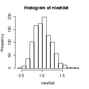
In Assignment #2, Chapter 4 Question C you looked at data giving the number of leaves on 53 plants and and you computed the variance-mean ratio to test whether it was overdispersed. Because you didn't know the sampling distribution of the variance-mean ratio, you could not do a test of significance or compute a P-value. Try the same simulation method you used to study the sampling distribution of the sample mean empirically in Assignment #1 Part C Question 2. Generate 1000 samples, each with 53 independent observations from a Poisson distribution with the same mean as the leaf data. Compute the variance-mean ratio for each sample, and use functions like max(), sort() and quantile() to see where the variance-mean ratio for the leaf data lies in this distribution. What would you give as a P-value in this case? Note that it is convenient to define a function vmratio() to compute the ratio.
> vmratio <- function(x) var(x)/mean(x)
> vmratio(nleaf)
[1] 2.269805
> nleafdat <- apply(matrix(rpois(53*1000,mean(nleaf)), ncol=1000), 2, vmratio)
> max(nleafdat)
[1] 1.866374
> quantile(nleafdat,c(0,.05,.1,.5,.9,.95,1))
       0%        5%       10%       50%       90%       95%      100%
0.4915865 0.7090018 0.7641761 1.0040652 1.2884700 1.3682384 1.8663744
> hist(nleafdat)

This is an empirical realization of the reference distribution, that is, the sampling distribution of the variance-mean ratio if the hypothesis of a Poisson distribution were true. We got it by generating 1000 realizations of the variance-mean ratio from a Poisson distribution with the same mean as that observed;. Since the observed ratio of 2.270 exceeds all of the 1000 values, the P-value is estimated to be < 0.001. Hence there is strong evidence from these data that the distribution of number of leaves is over-dispersed.