Data are taken from Example 13.4 on page 633 of Montgomery & Runger, Applied Statistics and Probability for Engineers, Second edition.
Aircraft primer paints are applied to aluminum surfaces by two methods; dipping and spraying. A factorial experiment was performed to investigate the effect of paint primer type and application method on paint adhesion. Adhesion force was measured, with three different primers and two application methods.
> paint <- data.frame(adhf = c(4.0,4.5,4.3,5.6,4.9,5.4,3.8,3.7,4.0,5.4,4.9,5.6,5.8,6.1,6.3,5.5,5.0,5.0),
 primer = factor(rep(rep(1:3,rep(3,3)),2)),applic = factor(rep(c("D","S"),c(9,9))))
> paint
   adhf primer applic
1   4.0      1      D
2   4.5      1      D
3   4.3      1      D
4   5.6      2      D
5   4.9      2      D
6   5.4      2      D
7   3.8      3      D
8   3.7      3      D
9   4.0      3      D
10  5.4      1      S
11  4.9      1      S
12  5.6      1      S
13  5.8      2      S
14  6.1      2      S
15  6.3      2      S
16  5.5      3      S
17  5.0      3      S
18  5.0      3      S
This is a one-way anova for primer, ignoring application method; lm() fits the linear model and anova() displayes the results in an anova table.
> anova(lm(adhf~primer, data=paint))
Analysis of Variance Table

Response: adhf
          Df Sum Sq Mean Sq F value  Pr(>F)
primer     2 4.5811  2.2906  5.5989 0.01527 *
Residuals 15 6.1367  0.4091
---
Signif. codes:  0 `***' 0.001 `**' 0.01 `*' 0.05 `.' 0.1 ` ' 1
This is a one-way anova for application method, ignoring primer.
> anova(lm(adhf~applic, data=paint))
Analysis of Variance Table

Response: adhf
          Df Sum Sq Mean Sq F value   Pr(>F)
applic     1 4.9089  4.9089  13.521 0.002039 **
Residuals 16 5.8089  0.3631
---
Signif. codes:  0 `***' 0.001 `**' 0.01 `*' 0.05 `.' 0.1 ` ' 1
This is a two-way anova for application method, primer and their interaction. Note that the sums of square for primer and for applic are the same as computed in the respective one-way analyses.
> anova(lm(adhf~primer*applic, data=paint))
Analysis of Variance Table

Response: adhf
              Df Sum Sq Mean Sq F value    Pr(>F)
primer         2 4.5811  2.2906 27.8581 3.097e-05 ***
applic         1 4.9089  4.9089 59.7027 5.357e-06 ***
primer:applic  2 0.2411  0.1206  1.4662    0.2693
Residuals     12 0.9867  0.0822
---
Signif. codes:  0 `***' 0.001 `**' 0.01 `*' 0.05 `.' 0.1 ` ' 1
The interaction is not significant (P = 0.27) so we can test the main effects, both of which are highly significant. We conclude that both the choice of primer and the choice of application method affect the adhesive force of the paint, and the differences between the three primers are the same with both application methods, and the difference between the two application methods is the same with each primer.
The summary shows the fitted coefficients and their t-tests.
> summary(lm(adhf~primer*applic, data=paint))

Call:
lm(formula = adhf ~ primer * applic, data = paint)

Residuals:
     Min       1Q   Median       3Q      Max
-0.40000 -0.16667  0.03333  0.21667  0.33333

Coefficients:
                Estimate Std. Error t value Pr(>|t|)
(Intercept)       4.2667     0.1656  25.772  7.1e-12 ***
primer2           1.0333     0.2341   4.414 0.000845 ***
primer3          -0.4333     0.2341  -1.851 0.088949 .
applicS           1.0333     0.2341   4.414 0.000845 ***
primer2:applicS  -0.2667     0.3311  -0.805 0.436265
primer3:applicS   0.3000     0.3311   0.906 0.382736
---
Signif. codes:  0 `***' 0.001 `**' 0.01 `*' 0.05 `.' 0.1 ` ' 1

Residual standard error: 0.2867 on 12 degrees of freedom
Multiple R-Squared: 0.9079,	Adjusted R-squared: 0.8696
F-statistic: 23.67 on 5 and 12 DF,  p-value: 7.89e-06
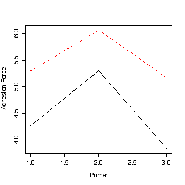
The next commands show how to compute means for the six different primer:applic combinations and how to arrange the means in a matrix to give the interaction plots.
> split(paint$adhf,paint$applic:paint$primer)
$"D:1"
[1] 4.0 4.5 4.3

$"D:2"
[1] 5.6 4.9 5.4

$"D:3"
[1] 3.8 3.7 4.0

$"S:1"
[1] 5.4 4.9 5.6

$"S:2"
[1] 5.8 6.1 6.3

$"S:3"
[1] 5.5 5.0 5.0

> sapply(split(paint$adhf,paint$applic:paint$primer),mean)
     D:1      D:2      D:3      S:1      S:2      S:3
4.266667 5.300000 3.833333 5.300000 6.066667 5.166667

> matrix(sapply(split(paint$adhf,paint$applic:paint$primer),mean),ncol=2)
         [,1]     [,2]
[1,] 4.266667 5.300000
[2,] 5.300000 6.066667
[3,] 3.833333 5.166667
matplot() plots each column of the matrix on the same graph.
> matplot(matrix(sapply(split(paint$adhf,paint$applic:paint$primer),mean),ncol=2),
type="l", xlab="Primer",ylab="Adhesion Force")
The two lines are close to parallel, confirming the conclusion of no interaction. That is, the differences between primers are the same for each application method.
> matplot(matrix(sapply(split(paint$adhf,paint$primer:paint$applic),mean),ncol=3),
type="l", xlab="Application",ylab="Adhesion Force")
You could also plot adhesion force against application method, with a different line for each primer. Again, the lines are close to parallel.