Questions
1. (a) Give John Tukey’s full name and state two of his statistical innovations.
(b) What two professions claim Florence Nightingale as a pioneer?
(c) Explain the difference between incidence and prevalence of a disease.
2. The following R code puts into a data frame the height of twin 1, the height of twin 2 and the zygosity (1 = mz, 2 = dz) of 12 pairs of twins, taken from the bone density study on Assignment #1, and plots three graphs. Sketch these graphs.
> twinht <- data.frame(ht1=c(159,169,160,168,154,161,162,165,150,159,163,162), ht2=c(162,169,161,167,160,160,160,159,156,150,158,162), zyg=c(1,1,1,1,1,1,2,2,2,2,2,2))
> attach(twinht)
> plot(ht1, ht2, pch=zyg)
> boxplot(split(ht1, zyg), xlab="Zygosity", ylab="Height of Twin 1")
> hist(ht1, breaks=c(150,155,165,170))
3. If a diagnostic score X follows a normal distribution with mean 60 and standard deviation 15 in the control group and a normal distribution with mean 40 and standard deviation 15 in the disease group, and a score of 45 or less is considered to be positive for the disease, what are the sensitivity and specificity of the test? If PV+ = 15%, what is the prevalence of the disease? Compute the Risk Ratio and Odds Ratio for the disease.
Note: F(1) = 0.8413447, F(1/3) = 0.6305587
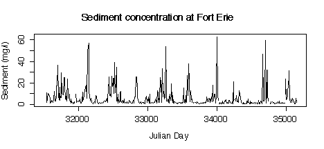
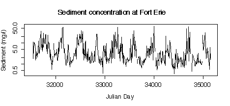
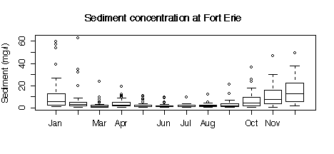
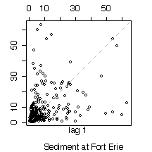
5. Here are five graphs from the Niagara Pollution Case Study data. The first shows the concentration of sediment in water (in mg/l) at Fort Erie as a time sequence plot over ten years, the second is the same but with concentration on a logarithmic scale. The third gives box plots by calendar month, the fourth is a lag-1 scatterplot, the fifth is a lag-1 scatterplot on a log scale. Discuss what you can learn from these graphs.

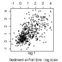
The R code used to create the plots is given here for your information; you are not expected to discuss the code in your answer.
> names(niagara)
[1] "station" "date" "julian" "disch" "sed" "die.w"
[7] "die.w.dl" "die.s" "die.s.dl" "pcb.w" "pcb.w.dl" "pcb.s"
[13] "pcb.s.dl"
> attach(niagara)
> plot(julian[station=="FE"],sed[station=="FE"],type="l", xlab="Julian Day",ylab="Sediment (mg/l)")
> title("Sediment concentration at Fort Erie")
> plot(julian[station=="FE"],sed[station=="FE"],type="l", xlab="Julian Day",ylab="Sediment (mg/l)",log="y")
> title("Sediment concentration at Fort Erie")
> months <- c("Jan","Feb","Mar","Apr","May","Jun","Jul","Aug","Sep","Oct","Nov","Dec")
> boxplot(split(sed[station=="FE"], substring(date[station=="FE"],4,6))[months], ylab="Sediment (mg/l)")
> title("Sediment concentration at Fort Erie")
> lag.plot(log(sed[station=="FE" & !is.na(sed)]))
> title(sub="Sediment at Fort Erie - log scale")
> lag.plot(sed[station=="FE" & !is.na(sed)])
> title(sub="Sediment at Fort Erie")