Statistics 2MA3 - Test #2 Solutions
2002-03-07 [Q2b solution revised 2002-03-14]
The marking scheme is indicated in red. Full Marks = 40.
Q1 [10]
- Give five interesting facts about the life and work of Siméon Denis Poisson (1781-1840). (Click here for pictures.)
- A parameter is a scalar or vector that indexes a family of probability distributions. A sample is a subset of observations selected from the population. A statistic is any function of the observations in a sample; it may not include any unknown parameters. The distribution of a statistic is called a sampling distribution; it describes how the statistic will vary from one sample to another.
Q2 [10]
- The distribution of X is discrete uniform, with each possible value from 1 to 6 having the same probabilty 1/6. Hence
E[X] = 1*(1/6) + 2*(1/6) + ... + 6*(1/6) = 3.5
E[X2] = 1*(1/6) + 4*(1/6) + ... + 36*(1/6) = 91/6
Var[X] = E[X2] - E[X]2 = 35/12 = 2.916667
- Since Y is the sum of 10 independent realizations of X, E[Y] = 10*E[X] = 35 and Var[Y] = 10*Var[X] = 350/12 = 29.16667. By the Central Limit Theorem the distribution of Y will be approximately normal so, approximately, P[Y > 45] = 1 - F((45.5 - 35)/sqrt(350/12)) = 0.02593. Note that I have used a continuity correction: because the actual score must be an integer, I have approximated the probability of getting 45 or less by taking the area under the normal curve up to 45.5. You will get a slightly different answer if you omit the continuity correction. Finally, the maximum score on any one die is 6 so we can say exactly that P[Y > 60] = 0.
Q3 [10]
> diedat
 [1] 3 6 3 6 4 4 2 5 3 6 2 3 6 5 1 5 3 3 5 3
> mean(diedat)
[1] 3.9
> var(diedat)
[1] 2.305263
> var(diedat)/mean(diedat)
[1] 0.5910931
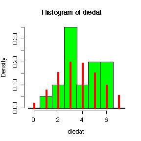
> hist(diedat,breaks=seq(-.5,7.5,by=1),prob=T,col="green")
> lines(0:7,dpois(0:7,mean(diedat)),lwd=3,type="h",col="red")
The data appear to be underdispersed, since the variance is much less than the mean. Compared to the Poisson distribution, the data are more concentrated in the range 1 to 6. [In fact, the data were generated to simulate 20 rolls of a 6-sided die.]

Q4 [10]
> diff <- (Lv2hrtrt-Bashrtrt)[Trtgrp=="P"]
> diff
 [1]  4 NA  5 NA  5 -8 NA -2  8  0 12 13  0  0 NA NA
> n <- sum(!is.na(diff))
> xbar <- mean(diff,na.rm=T)
> s <- sqrt(var(diff,na.rm=T))
> c(n=n, xbar=xbar, s=s)
        n      xbar         s
11.000000  3.363636  6.217278
> xbar + c(-1,1)*qt(.975,n-1)*s/sqrt(n)
[1] -0.8131878  7.5404605
> xbar + c(-1,1)*qnorm(.975)*s/sqrt(n)
[1] -0.3104726  7.0377453
- Whether computed as (-0.81, 7.54) with the t-distribution or, approximately, as (-0.31, 7.04) with the normal distribution, the 95% confidence interval for the mean difference in heart rate includes 0 so at the 95% level of confidence there is no evidence that the true mean difference between Level 2 heart rate and Baseline heart rate is not zero. This analysis assumes that the subjects are independent and the differences are normally distributed.
- The zero differences carry no information one way or the other; it would bias the result to treat them as positive or negative, so it is best to omit them and say that we have 6 positive differences out of 8 non-zero differences. Under the hypothesis that the median difference is zero, the number of positive differences will be distributed Bin(8, 0.5). The probability of getting 6 or more positive differences out of 8 would then be 28/256 + 8/256 + 1/256 = 0.1445 which is quite large so there is no reason to claim that the median difference between Level 2 heart rate and Baseline heart rate is not zero.

