Marks are indicated in red. Full marks = 100.
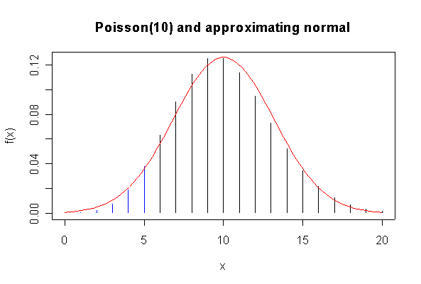
The N(10, 10) approximation to the Poisson(10) distribution is satisfactory graphically. The normal approximation to P(X <= 5) = 0.06709 is equally poor with (0.07736) or without (0.05692) the continuity correction.
> plot(0:20, dpois(0:20, 10), type="h", xlab="x", ylab="f(x)")
> lines(0:5, dpois(0:5, 10), type="h", col="blue")
> xgr <- seq(0, 20, len=80)
> lines(xgr, dnorm(xgr, 10, sqrt(10)), col="red")
> title(main="Poisson(10) and approximating normal")
> ppois(5, 10)
[1] 0.06708596
> pnorm(5.5, 10, sqrt(10))
[1] 0.07736446
> pnorm(5, 10, sqrt(10))
[1] 0.05692315
Note: I plotted normal density curves with the true mean and standard deviation, you could use fitted values if you prefer.
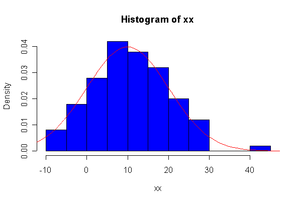
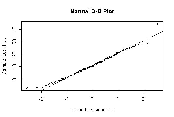
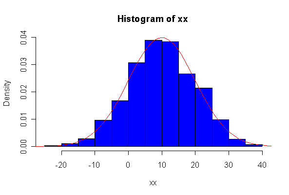
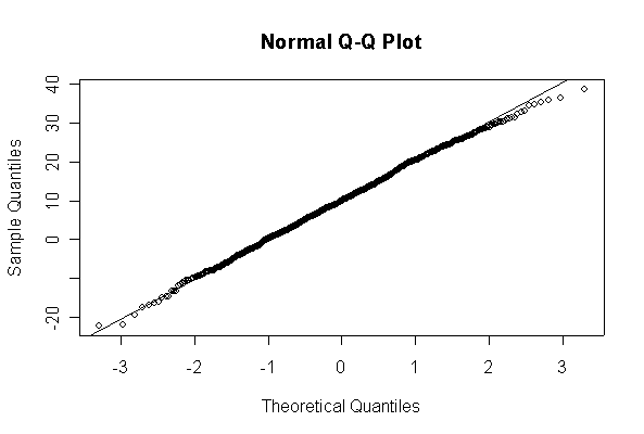
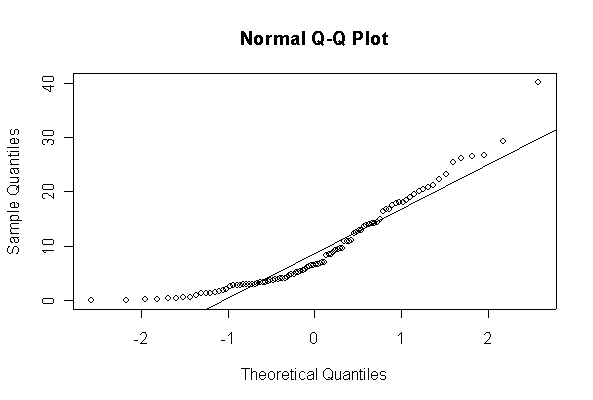
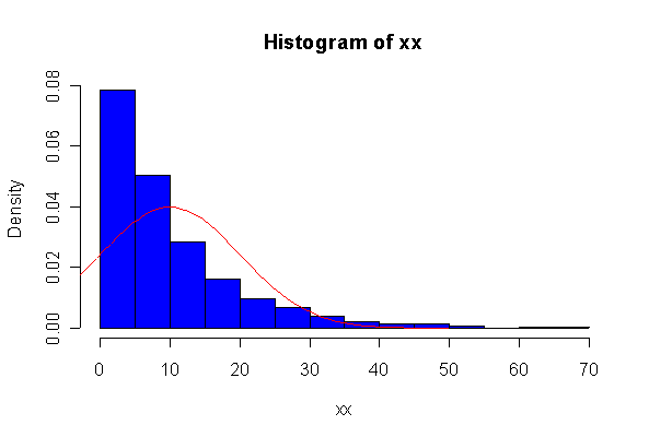
Not until n = 100 does the histogram begin to look Normal, and even then it is sometimes quite skewed. The Q-Q plot is reasonably straight when n = 40, except for the tails of the distribution. This suggests that at least 40 observations, but preferably 100 or more, are needed to demonstrate Normality.
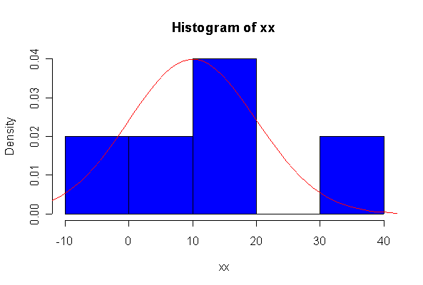
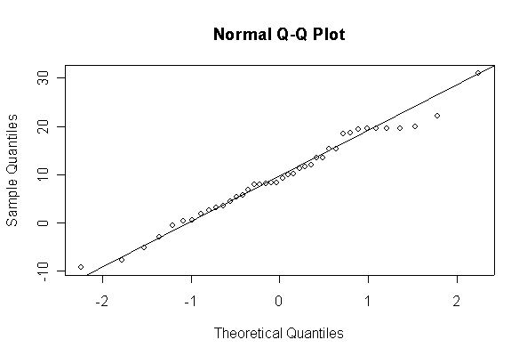
> xx <- rnorm(10, 10, 10)
> hist(xx, col="blue", prob=T)
> xgr <- seq(-50, 50, len=100)
> lines(xgr, dnorm(xgr, 10, 10), type="l", col="red")
> qqnorm(xx)
> qqline(xx)
Note: I plotted normal density curves with the true mean and standard deviation, you could use fitted values if you prefer.
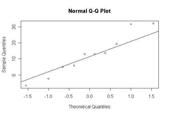
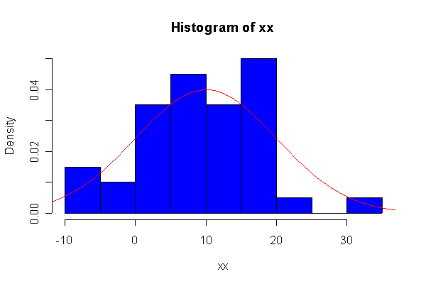
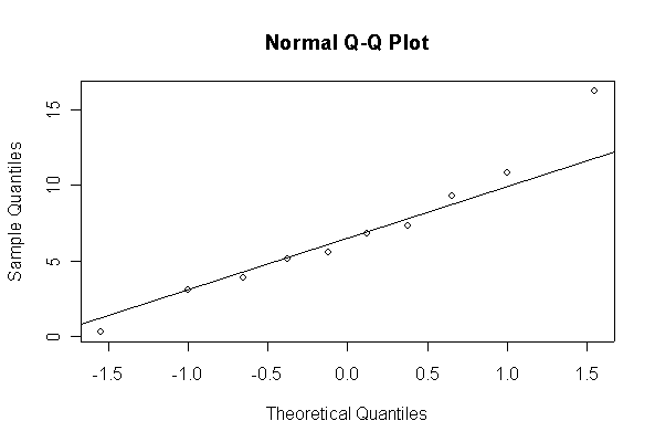
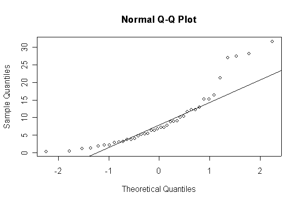
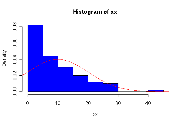
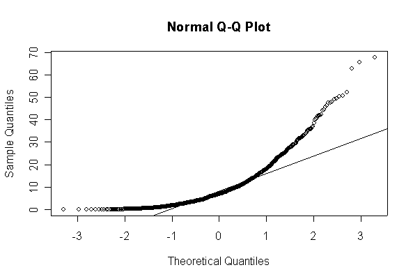
When n = 10 the histogram will often look as Normal, and the Normal Q-Q plot will often look as straight, as you would get with a Normal sample of the same size. When n = 40 or more, the histogram is consistently skewed and the Normal Q-Q plot shows a characteristic curvature that reliably indicates that the data did not come from a Normal distribution.
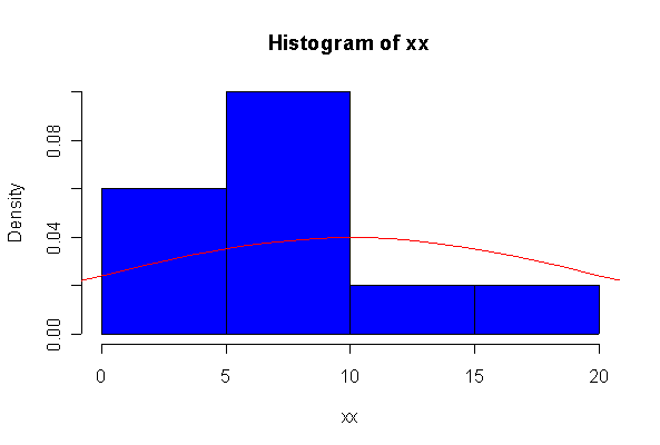
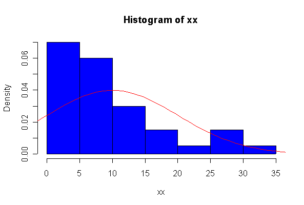
> xx <- rexp(10, 1/10)
> hist(xx, col="blue", prob=T)
> xgr <- seq(-50, 50, len=100)
> lines(xgr, dnorm(xgr, 10, 10), type="l", col="red")
> qqnorm(xx)
> qqline(xx)
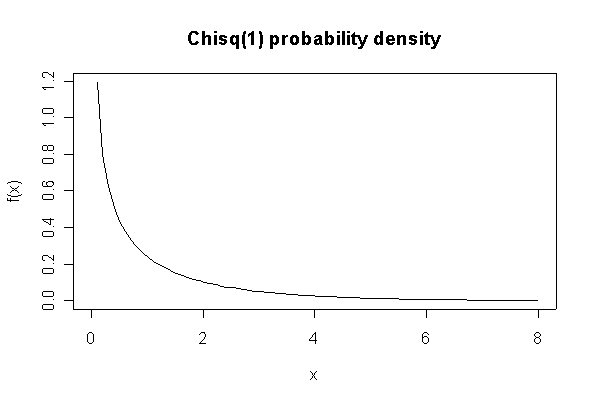
The chi-square distribution on 1 degree of freedom has mean = 1, standard deviation = 2. The general result that mean = df and sd = 2*df is given on page 262 of your text.
> plot(xgr, dchisq(xgr, 1), type="l", main="Chisq(1) probability density", xlab="x", ylab="f(x)")
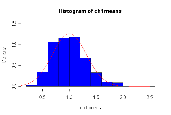
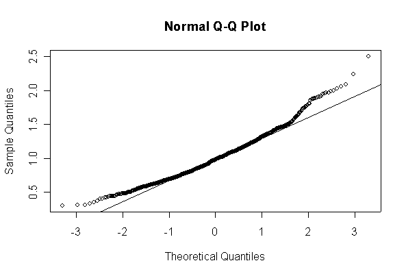
The Central Limit Theorem states that if n = 20, the distribution of the sample mean will be approximately Normal with mean = 1 and standard deviation = sqrt(2)/sqrt(20) = 0.3162278. If n = 200, the distribution of the sample mean should be even closer to Normal and have mean = 1 and standard deviation = sqrt(2)/sqrt(200) = 0.1.
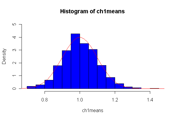
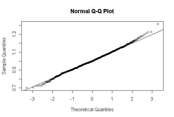
Here we have 1000 realizations of the sample mean. The histogram and Normal Q-Q plot indicate that the sampling distribution is very close to Normal, even though the data came from an extremely non-normal distribution. For n = 20, the observed mean of 1.005215 and standard deviation of 0.319037 are close to their theoretical values of 1 and 0.3162278, respectively. For n = 200, the observed mean of 1.003401 and standard deviation of 0.1010984 are close to their theoretical values of 1 and 0.1, respectively.
Note that I set the ylim of the histogram to make sure there would be room for the normal density, and I picked the grid for the normal density after I saw the histogram. I drew the normal density with the theoretical mean and standard deviation but you could use the fitted values, mean(ch1means) and sqrt(var(ch1means)).
> ch1means <- apply(matrix(rchisq(1000*20,1), ncol=20), 1, mean)
> length(ch1means)
[1] 1000
> mean(ch1means)
[1] 1.005215
> sqrt(var(ch1means))
[1] 0.319037
> hist(ch1means, col="blue", prob=T, ylim=c(0,1.5))
> xgr <- seq(0, 2.5, len=80)
> lines(xgr, dnorm(xgr, 1, sqrt(2/20)), col="red", type="l")
> qqnorm(ch1means)
> qqline(ch1means)
>
> ch1means <- apply(matrix(rchisq(1000*200,1), ncol=200), 1, mean)
> length(ch1means)
[1] 1000
> mean(ch1means)
[1] 1.003401
> sqrt(var(ch1means))
[1] 0.1010984
> hist(ch1means, col="blue", prob=T, ylim=c(0,5))
> xgr <- seq(0, 1.5, len=80)
> lines(xgr, dnorm(xgr, 1, sqrt(2/200)), col="red", type="l")
> qqnorm(ch1means)
> qqline(ch1means)
Define the events E (read error), S (skewed alignment) and O (off-centre alignment), and let ' denote complementary event.
We are given P(S) = 0.1, P(O) = 0.05 and P(SO) = 0.01, so we can compute P(SO') = P(S) - P(SO) = 0.09, P(S'O) = P(O) - P(SO) = 0.04, P(S'O') = 1 - P(SO') - P(S'O) - P(SO) = 0.86 to break down the problem into four mutually exclusive events.
Given that P(E|SO) = 0.06, P(E|SO') = 0.01, P(E|S'O) = 0.02, P(E|S'O') = 0.001, we can use total probability to compute the overall probability of a read error:
P(E) = P(E|SO)P(SO) + P(E|SO')P(SO') + P(E|S'O)P(S'O) + P(E|S'O')P(S'O') = 0.06*0.01 + 0.01*0.09 + 0.02*0.04 + 0.001*0.86 = 0.00316
Given that a read error occurred, the probability that the head is properly aligned is the conditional probability
P(S'O'|E) = P(E|S'O')P(S'O')/P(E) = 0.001*0.86 /0.00316 = 0.00086/0.00316 = 0.27215
Let X be the number of parts in a sample of 20 that need rework. Typically, X ~ Bin(20, 0.01), in which case E(X) = 0.2 and Var(X) = 0.198 so SD(X) = 0.445.
(a) If X exceeds its mean by more than 3 standard deviations, X > 1.535, but because X is integer-valued P(X > 1.535) = P(X > 1) = 1 - P(X <= 1) = 0.01686
(b) Now X ~ Bin(20, 0.04) so P(X > 1) = 1 - P(X <=1) = 1 - 0.8103 = 0.1897
(c) Let W be the number of hours out of the next 5 in which parts need rework. Assuming that the hours are independent, W ~ Bin(5, P(X > 1)) where, again, X ~ Bin(20, 0.04). The required probability is thus
P(W >= 1) = 1 - P(W = 0) = 1 - [1 - P(X > 1)]^5 = 1 - P(X <= 1)^5 = 1 - (0.8103)^5 = 0.6506
> 1-pbinom(1, 20, .01)
[1] 0.01685934
> pbinom(1, 20, .04)
[1] 0.8103378
> 1-pbinom(1, 20, .04)
[1] 0.1896622
> 1-pbinom(1, 20, .04)^5
[1] 0.6505939
> 1 - pbinom(0, 5, 1-pbinom(1, 20, .04))
[1] 0.6505939
Let n be the total number of components on hand and let X be the number that are not defectived, so X ~ Bin(n, 0.98). An order for 100 components can be filled without reordering if X >= 100. I have used R here but you should also know how to do these calculations on your calculator.
(a) If n = 100, P(X >= 100) = 0.133
(b) If n = 102, P(X >= 100) = 0.666
(c) If n = 105, P(X >= 100) = 0.981
> 1 - pbinom(99, 100, .98)
[1] 0.1326196
> 1 - pbinom(99, 102, .98)
[1] 0.6657502
> 1 - pbinom(99, 105, .98)
[1] 0.9807593
Let X be the number of asbestos fibers in one grid cell. From the numbers given, the mean number of asbestos fibers in one grid cell is 800*100/160000 = 0.5, so X ~ Pois(0.5).
(a) P(X >= 1) = 1 - P(X = 0) = 1 - exp(-0.5) = 0.3935
(b) The number of cells that need to be observed to find 1 with fibres will follow a geometric distribution with mean = 1/P(X >= 1) = 1/0.3935 = 2.541, so the mean number of cells that need to be observed to find 10 cells with fibers will be 10 times that, i.e. 25.41.
(c) The variance of the geometric distribution will be (1 - 0.3935)/(0.3935^2), so the variance number of cells that need to be observed to find 10 cells with fibers will be 10 times that, i.e. 10*(1 - 0.3935)/(0.3935^2) = 39.177, hence the standard deviation is 6.259.
> 1-dpois(0,.5)
[1] 0.3934693
> 10/(1-dpois(0,.5))
[1] 25.41494
> 10*dpois(0, .5)/(1-dpois(0,.5))^2
[1] 39.17698
> sqrt(10*dpois(0, .5)/(1-dpois(0,.5))^2)
[1] 6.259152
The specifications require that the dot diameter be within the range 0.0020 +/- 0.0006 inches with probability 0.9973. Assume that the dot diameter is normally distributed. A normal random variable will be within 3 standard deviations of its mean with that probability, so the standard deviation must be sigma = 0.0002.
To find this with the tables, taking the left tail, you need F((0.0014 - 0.002)/sigma) = (1 - 0.9973)/2 = 0.00135; interpolating in Table II gives F(-3.00) = 0.00135, so just solve for sigma in the equation (0.0014 - 0.002)/sigma = -3 to get sigma = 0.0002. Note that I have verified the result by showing that sigma = 0.0002 gives the correct probability for the interval given.
> qnorm((1-0.9973)/2)
[1] -2.999977
> pnorm(0.0026, 0.002, 0.0002) - pnorm(0.0014, 0.002, 0.0002)
[1] 0.9973002
Let X be the diameter of a given bearing. We are given that X ~ N(1.5, 0.025^2), so the probability that a given bearing does not exceed 1.6 mm is P(X < 1.6) = F((1.6 - 1.5)/0.025) = F(4) = 0.9999683. The maximum diameter of the 10 bearings will not exceed 1.6 mm if and only if all 10 have diameters less than 1.6 mm. Since they are assumed independent, the probability of this happening is F(4)^10 so the required answer is that the probability that the largest of the 10 exceeds 1.6 mm is 1 - F(4)^10 = 0.000317.
Since F(4) is off the table in the book, you have to use the computer or find a better table.
[Note that you could have got almost the correct answer by taking the probability that a given bearing exceeds 1.6 mm and multiplying by 10. Why is this incorrect? Why does it give almost exactly the same numerical value?]
> pnorm(4)
[1] 0.9999683
> 1 - pnorm(4)
[1] 3.167124e-05
> 1 - pnorm(4)^10
[1] 0.0003166673
> 10*(1 - pnorm(4))
[1] 0.0003167124